Architecting scalable checkpoint storage for large-scale ML training on AWS

The exponential growth in size and complexity of foundation models (FMs) has created unprecedented infrastructure demands across compute, networking, and storage resources. Storage systems, in particular, face intense requirements for throughput, latency, and capacity. In machine learning (ML) model training, these storage demands are particularly evident in checkpointing—a critical reliability mechanism that periodically saves and restores model states, placing enormous strain on storage infrastructure. This process necessitates high-performance storage systems capable of rapidly reading and writing terabytes of data, such as model parameters and optimizer state, both from and to persistent storage without creating training bottlenecks. As model sizes continue to grow, the storage throughput and capacity requirements for efficient checkpointing operations increase proportionally.

As organizations scale their ML training to thousands of accelerators, system disruptions become statistically inevitable, making checkpointing crucial for protecting training progress and enabling recovery. However, the process of saving these checkpoints introduces computational overhead that can significantly impact training efficiency. For example, in large language model (LLM) training with 4,000 accelerators, inefficient checkpointing can waste thousands of GPU hours daily, directly affecting training costs and time to production. This makes checkpoint optimization essential for maintaining productivity in large-scale ML training operations.

In this post, we focus on optimizing checkpoint operations for LLM training, where workloads are highly demanding at the petabyte scale. We explore architectural patterns and practical strategies for building robust storage infrastructures, using checkpoint optimization as a foundational technique. Our guidance emphasizes balancing performance, scalability, and cost-effectiveness in checkpoint operations.

Storage infrastructure for large-scale ML training

To support efficient checkpoint operations and overall training performance in large-scale ML workloads, organizations need robust storage infrastructure. This section explores key storage infrastructure options for effective checkpointing at scale. In FM training, Amazon Web Services (AWS) users have successfully adopted several storage patterns, typically grouped into three categories:

• Amazon S3: Many users start by aggregating their data in Amazon S3, using its 99.999999999% (11 nines) data durability, cost-effectiveness, and virtually unlimited capacity. Amazon S3 provides broad integrations with both AWS and partner services for data ingestion, integration, cataloging, and processing. Users often optimize costs by using the Amazon S3 Intelligent-Tiering storage class for automatic data movement between access tiers, while others use Amazon S3 Express One Zone storage class for single-digit millisecond latency access to frequently accessed data, which can be particularly beneficial for iterative ML training workloads needing rapid data access.
• Amazon FSx for Lustre: This pattern uses FSx for Lustre for POSIX-compliant file system access. FSx for Lustre delivers sub-millisecond latencies and throughput of up to hundreds of gigabytes per second, making it well-suited for feeding data to resource-intensive ML clusters. Recently, Amazon FSx for Lustre launched the Intelligent-Tiering storage class, which delivers virtually unlimited scalability, fully elastic Lustre storage, and the lowest-cost Lustre file storage in the cloud. FSx for Lustre Intelligent-Tiering automatically scales storage up or down based on access patterns and optimizes costs by tiering between Frequent Access, Infrequent Access, and Archive tiers. For latency-sensitive workloads, an optional SSD read cache delivers high performance for frequently accessed data.High-performance networking is essential for effective ML training at scale. Elastic Fabric Adapter (EFA) provides ultra-low latency networking for two critical aspects of distributed training: efficient distribution of model checkpoints across machines and rapid collective operations for data sharing during training. These high-performance networking capabilities are particularly valuable when implementing hierarchical checkpoint distribution. This is an access pattern that we examine later in this post that enhances the efficiency of any storage solution by optimizing how checkpoint data flows throughout the training cluster.
• Hybrid approach: Some users combine Amazon S3 and FSx for Lustre in a multi-tiered storage architecture, using the strengths of each service for different aspects of their ML workflows.

Checkpoint fundamentals

The following sections outline the checkpoint fundamentals.

Checkpointing operations and training efficiency

Checkpointing protects against failures and enables point-in-time training resumption when interruptions occur. As we scale ML training to thousands of accelerators, the optimal balance between checkpointing frequency and system failures becomes critical. When we talk about checkpoint overhead, we’re referring to several resource costs: the computational pauses required to save model states, the storage I/O operations needed to write and read checkpoint data, and the network bandwidth consumed during these processes. All of these factors can temporarily reduce or halt productive training computation. Frequent checkpoints offer better protection against failures but increase this overhead, while infrequent checkpoints reduce overhead but risk losing more computation time when failures occur. Therefore, organizations must weigh the total time spent checkpointing against the potential computation time lost to failures. To quantify this impact and optimize our checkpointing strategies, we need a metric that captures the true productivity of our training operations. This is where the concept of “ML Productivity Goodput” becomes crucial.

Traditional goodput measures the amount of application-level data successfully transmitted over a network per unit of time (excluding protocol overhead and retransmitted data). However, ML training adapts this concept. In ML training, the Runtime Goodput metric measures the fraction of time spent on actual training progress as compared to the total time when compute resources are allocated and ready for training. This metric provides a more accurate measure of actual productivity than raw throughput metrics by excluding overhead data. The following figure shows a theoretical model showing how increasing cluster size negatively impacts ML productivity goodput due to higher system failure probability. Various checkpointing strategies show different conceptual efficiency outcomes at scale. This illustration represents a simplified analytical model rather than empirical measurements. As cluster size increases, the probability of system failures grows, reducing training efficiency. Different checkpointing strategies have varying impacts on training efficiency as scale increases. The “No Checkpointing” line in Figure 1 represents an idealized scenario where we calculate expected goodput by factoring in the statistical likelihood of failures at different scales. This calculation assumes that when a failure occurs without checkpointing, all progress since the beginning of training is lost, requiring a complete restart. At smaller scales where failures are relatively rare, this can still yield reasonable goodput (near 80%), as most training runs complete successfully. However, as scale increases, the probability of experiencing at least one failure before training completion rises dramatically, causing the steep decline in expected goodput. Synchronous checkpointing, which has been the standard approach in ML frameworks for many years, creates more significant training interruptions, while newer optimized approaches that minimize training pauses can help maintain higher goodput, especially at scale. We explore these optimization techniques in detail, such as asynchronous checkpointing, later in this post.

Figure 1: Impact of cluster size on ML Productivity Goodput

Scale introduces significant reliability challenges. As compute clusters grow, failures become more frequent due to the mathematics of system reliability. In a distributed system with thousands of components, the cluster-wide mean time between failures (MTBF) decreases inversely proportional to the number of components. For example, if individual compute nodes have a 0.1% daily failure probability (corresponding to a 1,000-day MTBF per node), a 500-node cluster would experience a system-wide MTBF of just 2 days (1,000 ÷ 500). With 4,000 accelerators across these nodes, component-level issues like GPU memory errors, network timeouts, or local storage failures become statistically inevitable on a daily or even hourly basis. This dramatic reduction in MTBF directly impacts training continuity and increases the importance of efficient checkpoint-restore capabilities to maintain productive training operations. This makes checkpointing essential for maintaining acceptable goodput levels. Checkpointing operates through two paths:

• Write path: Periodically captures snapshots of training state—such as model parameters, optimizer state, learning rate schedulers, and metrics—saving them to durable storage. This process in standard implementations acts as a synchronous barrier in training, necessitating that all computation pause while writing the checkpoint.
• Read path: Restores saved state for recovery or model fine-tuning by reloading parameters and reconfiguring the training environment.

Although they’re essential for reliability, both checkpointing operations can create significant overhead in distributed training of large models. This necessitates optimizations such as asynchronous checkpointing and efficient storage architecture to maximize training efficiency and cost-effectiveness.

The size, frequency, and distribution patterns of your checkpoint operations directly influence your optimal storage architecture. As model size increases from billions to trillions of parameters, and as training clusters scale from dozens to thousands of accelerators, storage requirements evolve from simple direct access patterns to sophisticated multi-tiered architectures. Understanding these scaling factors is crucial for selecting appropriate storage technologies and implementing efficient checkpoint distribution patterns.

Checkpoint sizing

Checkpoint size is a critical factor in planning infrastructure for LLM training. The size of a checkpoint depends on three key factors:

• Model parameters
• World size (cluster size)
• Distributed training techniques such as model parallelism (MP) or data parallelism (DP)

The base checkpoint size comes from the storage needed for model parameters. With two bytes for the parameter itself (stored as BF16/FP16) and eight more bytes for the optimizer state, each parameter typically needs 10 bytes of storage in a checkpoint during training. Although checkpoint size primarily depends on model parameters, both world size and distributed training techniques influence the total storage requirements needed for checkpoints.

World size refers to the total number of accelerators in the training cluster, where a cluster consists of multiple compute nodes, and each node contains multiple accelerators.

The distributed training techniques influence how checkpoints are stored and accessed. The following are two key approaches:

• Model parallelism splits a single model across multiple accelerators (called ranks) when the model exceeds the memory capacity of a single accelerator.
• Data parallelism creates multiple copies (called replicas) of the same model and trains each copy on different portions of the training data simultaneously.

To calculate checkpoint sizes for LLM training, we can use the following formulas:

Basic checkpoint size formula:

Single Model Replica (MR) Checkpoint Size = (P × Wp) + (P × Os)
Where:
P = Number of total model parameters
Wp = Storage per parameter for weights (typically 2 bytes for BF16/FP16)
Os = Storage per parameter for optimizer state (typically 8 bytes)

Distributed training storage requirements:

Total Checkpoint Write Size = Single MR Checkpoint Size
Total Checkpoint Read Size = Single MR Checkpoint Size × Number of MRs
Where:
Number of MRs = Total Accelerators ÷ Accelerators Per MR

To calculate checkpoint sizes, we can use an example: a 100-billion-parameter model training on a 4,000-accelerator cluster:

Cluster configuration:

• • Total accelerators: 4,000
  • Total nodes: 500 (Each node is configured as an instance with eight accelerators)
  • Accelerators per MR: 32
  • Data parallelism (DP) degree: 125 (= 4,000 total accelerators ÷ 32 accelerators per MR). This represents the number of MRs in the cluster.

Model checkpoint size:

• • Total model parameters: 100 billion (100B)
  • Parameter weights (BF16): 200 GB (= 100 B parameters × 2 bytes)
  • Optimizer state: 800 GB (= 100B parameters × 8 bytes)
  • Single checkpoint size per MR: 1 TB (= 200 GB + 800 GB)
  • Total checkpoint data to read across all MRs: 125 TB (= 125 MR × 1 TB/MR). Each MR must load the complete 1 TB checkpoint as part of the training initialization process before training resumes.
  • Total checkpoint data to write: 1 TB (= 200 GB + 800GB). In data-parallel distributed training, all MRs maintain identical parameters through synchronization during the optimization step. After each batch, gradients from all replicas are aggregated (typically via all-reduce operations), ensuring that when a checkpoint is saved, any single replica contains the complete, synchronized model states. This synchronization means we only need to save one replica’s state rather than saving each replica separately.

This mathematical relationship between model parameters and checkpoint size helps us understand the storage requirements for our training infrastructure. However, when scaling to thousands of accelerators, the challenge isn’t just about storage capacity—it’s about managing concurrent access to these massive checkpoints.

Checkpointing reading strategies at scale

Reading checkpoints involves loading saved snapshots of the model states from storage to resume or continue training. The primary objective when reading checkpoints is to minimize the time spent reading and deserializing the model state data, as this directly impacts training resumption latency and system efficiency. There are two approaches to reading checkpoints at scale: concurrent loading and hierarchical distribution. The choice between concurrent loading and hierarchical distribution depends on three key factors: world size, checkpoint size, and loading time requirements.

Concurrent loading is generally more suitable for smaller deployments and smaller checkpoints (under 100 GB), where longer loading times (5+ minutes) are acceptable. The point at which concurrent loading becomes inefficient depends on multiple factors, such as instance network bandwidth, storage throughput limitations, checkpoint size, and cluster network topology. As cluster sizes scale, the simultaneous demand on shared storage resources and network paths typically leads to increasing contention and throughput limitations. Organizations should evaluate their specific infrastructure configuration to determine the optimal threshold for switching from concurrent loading to hierarchical distribution.

Concurrent loading

When hundreds of accelerators attempt to load checkpoints simultaneously, the situation creates unique challenges that can destabilize the training infrastructure. In our preceding example, consider a cluster with 4,000 accelerators across 500 nodes, where all accelerators initialize training simultaneously. This synchronized demand creates massive spikes across shared network links, causing Storage bottlenecks that negatively impact checkpoint loading time.

If our target is to load the total checkpoint data of 125 TB in two minutes to the cluster, then the throughput on the storage system with concurrent scaling would be approximately 8.3 Tbps (125 TB ÷ 120 seconds = 1,042 GB/second = 8,333 Gbps). This necessitates substantial network capacity. Regardless of the underlying storage solution—whether Amazon S3, Amazon S3 Express One Zone, or FSx for Lustre—concurrent loading at this scale creates intense demand spikes that need careful management of network bandwidth, storage throughput limits, and connection resources. This includes implementing retry mechanisms with exponential backoff, properly configuring connection pools, and monitoring for throttling or congestion across both storage and network pathways. These synchronized demand spikes can create storage bottlenecks that negatively impact checkpoint loading time if they exceed service-specific limits, regardless of whether you’re using Amazon S3, Amazon S3 Express One Zone, or FSx for Lustre.

Storage solutions such as Amazon S3 Express One Zone Storage Class or FSx for Lustre provide high-performance file system access with throughput of hundreds of gigabytes per second. At large scale with thousands of accelerators, concurrent loading of terabyte-sized checkpoints (such as the 1 TB per MR example we discussed previously) typically results in end-to-end loading times of 10-15 minutes. This loading time is affected by factors including metadata operations and network traffic patterns when many clients access storage simultaneously. For time-sensitive training workloads, this duration can impact overall training efficiency, motivating exploration of alternative distribution patterns.

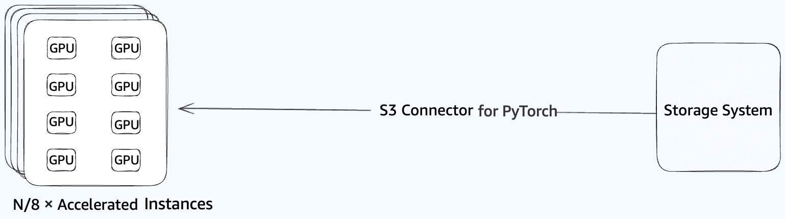
Figure 2: Amazon S3 storage connection to GPU cluster for concurrent PyTorch checkpoint loading

Hierarchical distribution

An effective approach to reduce network spikes is implementing a hierarchical distribution system for checkpointing to help extract better performance from the storage system. In this approach, designated leader nodes first load the checkpoint from the storage system. In both concurrent loading and hierarchical distribution, MP means each accelerator only needs a specific portion of the checkpoint corresponding to its assigned model shard. The key difference is in how this data flows: with concurrent loading, all nodes independently access storage to retrieve their portions, creating multiple forms of contention (including network congestion at shared connection points, throughput bottlenecks from service limits, and possible metadata hotspotting when accessing similar objects); with hierarchical distribution, only leader nodes retrieve data from storage, and then use EFA to efficiently distribute these portions to other worker nodes responsible for the same model shard. This strategy dramatically reduces the direct load on the storage system while using the high-performance networking capabilities of EFA.

Using our earlier example, if our target is to load the total checkpoint data of 125 TB in 2 minutes to the 4,000-accelerator cluster, hierarchical distribution significantly reduces the load on the storage system compared to concurrent loading. While concurrent loading would require approximately 8.3 Tbps (125 TB ÷ 120 seconds = 1,042 GB/second = 8,333 Gbps) from the storage system, hierarchical distribution needs only approximately 66.7 Gbps from storage (1 TB ÷ 120 seconds = 8.33 GB/second = 66.7 Gbps). This 125x reduction in storage throughput requirements makes the 2-minute checkpoint loading goal consistently achievable, even at massive scale. Then, the leader nodes efficiently distribute the data to the rest of the cluster using the high-performance EFA network, which we explain in more detail in the next section.

The hierarchical distribution approach uses the high-bandwidth, low-latency networking infrastructure available within modern accelerator clusters to efficiently distribute checkpoint data. This approach takes advantage of the network topology where intra-cluster communication typically offers significantly higher bandwidth than connections to external storage services. By limiting external storage access to just the leader nodes and then distributing data efficiently within the cluster’s high-performance network fabric, this method dramatically reduces overall storage access requirements. The checkpoint distribution uses collective communication operations optimized for this purpose, enabling efficient data movement between leader and worker nodes throughout the cluster.

The following figure shows the hierarchical distribution approach for checkpoint reading. In our calculations, let n = 32 be the number of accelerators needed for one complete model split in MP, and let N = 4,000 be the total number of accelerators in the training cluster. Each instance contains eight accelerators, thus n/8 = 4 instances are needed for leader nodes to read from storage and hold one complete model split, while N/8 – n/8 = 496 instances are for worker nodes to receive the checkpoint data. The checkpoint distribution uses NVIDIA Collective Communications Library (NCCL) broadcast, enabling efficient communication between leader and worker nodes.

Figure 3: Hierarchical checkpoint distribution architecture using NCCL broadcast

The hierarchical distribution reduces external network throughput demands by a factor equal to the data parallelism degree (125 in our example). This approach significantly decreases the risk of network congestion and potential throughput limitations when accessing external storage systems, regardless of the specific storage technology employed. Maximizing data transfer over the optimized high-throughput network within the compute cluster allows this approach to enable faster checkpoint reading through efficient use of network topology and bandwidth.

When implementing hierarchical checkpoint distribution, your choice of external storage technology that serves checkpoint data to the leader nodes significantly impacts overall performance. The required Storage performance depends on factors including checkpoint size, frequency, and the number of leader nodes accessing storage simultaneously. While this architectural pattern reduces direct storage access requirements by a factor equal to your data parallelism degree, the leader nodes still need sufficient throughput to load checkpoints within your target time window. In the follow-up post, we’ll explore specific AWS storage technologies optimized for this access pattern.

Checkpointing writing strategies at scale

Writing checkpoints involves saving snapshots of the model states to storage during training. The primary goal when writing these checkpoints is to minimize training interruption while making sure of reliable state persistence. During checkpoint writing, computational pauses occur when the training process stops to save the model states, which directly impacts accelerator usage and costs.

In large distributed training clusters, checkpoint writing can follow different patterns. In some implementations, particularly for data-parallel training, a single designated rank (often rank 0) might aggregate and write the entire model checkpoint. In other cases, especially with model-parallel training where different accelerators hold different portions of the model, each participating rank might write its own portion of the checkpoint. The optimal approach depends on the distributed training strategy in use, with considerations for both model and data parallelism affecting the checkpoint writing pattern.

A critical design decision in checkpoint writing is determining the checkpoint frequency — how often we should save checkpoints during training. Checkpoint frequency must balance failure recovery needs with training efficiency to maintain optimal goodput, enhancing the ratio of actual productive computation achieved to total resource usage. In large-scale distributed environments, as world size increases, failures are statistically inevitable and the mean time between failures decreases linearly. This necessitates more frequent checkpoints to limit potential lost progress and computational work while managing checkpoint overhead.

Beyond frequency, understanding how checkpoint writing differs from reading is crucial for optimizing the process. Our previous example demonstrates this asymmetry: reading necessitates distributing 125 TB across all MRs (125 MR × 1 TB/MR), while writing can follow different patterns. For pure data-parallel training with smaller models, writing often needs only 1 TB from a single replica to capture the complete model states. However, alternative approaches exist where each accelerator writes its own portion of the model checkpoint, which is particularly common in model-parallel training where different accelerators hold different parts of the model. This approach may be preferred when working with extremely large models that benefit from parallel I/O operations during checkpoint writing.

In the next section we examine synchronous and asynchronous checkpoint writing approaches to understand their impact on training efficiency.

Synchronous checkpointing

In traditional synchronous checkpointing, the entire training process must pause while model states are saved to storage. When performed across thousands of instances, these synchronous checkpoint writes become expensive in terms of storage and network throughput. For large models such as our 100 B-parameter model example, this pause can extend to several minutes, leaving all accelerators in the cluster idle.

In a 4,000-accelerator cluster, a three minute pause for each synchronous checkpoint write means 200 GPU-hours of cluster-wide idle time (4,000 accelerators × 3 minutes = 12,000 minutes = 200 GPU-hours). When checkpoints are saved every 30 minutes during training, the cluster spends 2.4 hours per day in checkpoint idle time (48 daily checkpoints × 3 minutes = 2.4 hours), adding up to 9,600 cluster-wide GPU-hours lost daily (2.4 hours × 4,000 accelerators) to checkpointing alone. Even though only one MR (32 accelerators) needs to write checkpoint data, this synchronous checkpointing creates an intense spike in storage and network I/O that forces all 4,000 accelerators in the cluster to halt training during the write operation.

Asynchronous checkpointing

Asynchronous writes address the training interruptions and I/O spikes by allowing the training process to continue while checkpoints are staged and saved in the background. Instead of halting training during storage I/O, the training process quickly copies model states into a separate staging buffer and immediately resumes computation. Then, a background process handles the I/O operations to persist these model states from the staging buffer into storage as checkpoint data, transforming idle accelerator time into productive training time.

PyTorch v2.4.0+ implements this concept through DCP’s asynchronous saving feature, which helps reduce bottlenecks in distributed training workloads by enabling parallel checkpointing. As described in the “Asynchronous Saving with Distributed Checkpoint” post, DCP offers two approaches: a basic version using CPU buffers and an optimized version using pinned memory. The basic version copies model states to CPU buffers for asynchronous processing but demands careful memory management, as CPU usage increases with checkpoint size and number of accelerators. The pinned memory version improves performance by using a persistent buffer for checkpoint staging, but sustains peak memory pressure throughout the application’s lifecycle.

The required Storage performance for asynchronous checkpointing depends primarily on model size, which directly determines checkpoint size as we established earlier. Since larger models (with parameters in the hundreds of billions or trillions) generate correspondingly larger checkpoints (often measured in terabytes), they require storage solutions with higher throughput for sequential writes and efficient handling of large objects. Additionally, as model size increases, organizations typically deploy larger clusters to maintain reasonable training times, which in turn increases failure probability and necessitates more frequent checkpoints. This creates a compounding effect: larger models need both larger and more frequent checkpoints, placing even greater demands on storage infrastructure. For FMs with hundreds of billions of parameters, high-throughput object storage or parallel file systems with burst capacity in the hundreds of GB/s range are typically required to handle these intensive I/O patterns. Our follow-up post will examine specific AWS storage technologies and their performance characteristics based on model size tiers, helping you match your storage architecture to your specific model scale.

Multi-level checkpointing

While asynchronous checkpointing helps minimize training interruptions, we can further optimize checkpoint operations through multi-level checkpointing—a strategy that complements our hierarchical distribution and asynchronous approaches. Multi-level checkpointing creates checkpoints at different frequencies across multiple storage tiers, each with distinct performance characteristics and durability guarantees. Multi-level checkpointing addresses a fundamental challenge in large-scale training: frequent checkpoints are desirable for minimizing lost work during failures, but writing each checkpoint to durable storage creates significant I/O overhead. By leveraging a hierarchy of storage systems with different performance-durability tradeoffs, we can create more frequent lightweight checkpoints for quick recovery scenarios while reserving durable storage operations for less frequent but more critical persistence points.

In a typical multi-level checkpointing implementation for ML training on AWS, we might define:

• Fast-tier checkpoints: Created very frequently (every few minutes) and stored in high-speed, local media such as instance memory, GPU memory, or local NVMe storage. These checkpoints provide rapid recovery from transient failures that don’t affect the local storage itself, such as application crashes, out-of-memory errors, numerical instabilities (e.g., NaN gradients), or temporary network partitions. In these scenarios, the compute instance remains operational and local storage remains intact, allowing quick recovery without accessing external storage systems. However, these checkpoints offer limited durability since they exist only on the local node and cannot protect against hardware failures, instance terminations, or availability zone issues.
• Durable-tier checkpoints: Created less frequently (hourly or at significant training milestones) and stored in highly durable storage such as Amazon S3 or FSx for Lustre. These protect against complete cluster failures, availability zone issues, or scheduled infrastructure events.

For our earlier example of a 100B-parameter model training on 4,000 accelerators, this approach significantly improves overall training performance and reduces costs. By minimizing the frequency of expensive I/O operations to shared storage services while maintaining strong recovery capabilities, you can achieve faster training throughput and lower your storage operation costs. The training process might create fast-tier checkpoints every 5 minutes, mid-tier checkpoints every 30 minutes, and write to durable storage like Amazon S3 only once every few hours. This tiered approach maximizes GPU utilization by keeping accelerators computing rather than waiting on I/O operations, which directly translates to shorter time-to-model completion and lower infrastructure costs. When implemented alongside our hierarchical distribution and asynchronous checkpointing techniques, multi-level checkpointing completes a comprehensive checkpoint optimization strategy that balances performance, recovery capabilities, and resource efficiency at scale.

Implementation walkthrough for checkpoint optimization

Implementing hierarchical distribution and asynchronous checkpointing patterns works with either Amazon S3/Amazon S3 Express One Zone or FSx for Lustre as your storage foundation. The core logic remains consistent across storage options, with minor configuration differences:

Implementation using Amazon S3, Amazon S3 Express One Zone, or Amazon FSx for Lustre

As with the standard pattern, we start by identifying leader nodes:

# Step 1: Define helper functions to identify leader nodes
def get_model_parallel_rank(rank, model_parallel_size):
    return rank % model_parallel_size

def is_worker_on_leader_replica_host(rank, workers_per_host, model_parallel_size):
    return get_model_parallel_rank(rank, model_parallel_size) < workers_per_host

Once we’ve identified the leader nodes, they use PyTorch’s Amazon S3 connector to read checkpoint data from your preferred storage. Note the URL format for Amazon S3 Express One Zone includes zone information, and we have included multiple snippets for each storage solution:

# Step 2: Leaders read from storage - configuration varies by storage type
rank = dist.get_rank()
model_parallel_size = 32  # GPUs per complete model replica
workers_per_host = 8      # Number of workers per host instance

if is_worker_on_leader_replica_host(rank, workers_per_host, model_parallel_size):
    import torch.distributed.checkpoint as DCP
    from s3torchconnector import S3ClientConfig
    from s3torchconnector.dcp import S3StorageReader

    # For Amazon S3 Express One Zone (single-digit ms latency)
    config = S3ClientConfig(
        part_size=100 * 1024 * 1024,    # Smaller parts work well with Express One Zone's low latency
        throughput_target_gbps=15,      # Throughput target in Gbps, determines number of connections
        max_attempts=10                 # Number of retries for retriable errors
    )

    # Load checkpoint from Amazon S3
    reader = S3StorageReader(
        region="us-east-1", 
        path="s3://your-checkpoint-bucket--azid--use1-az1--x-s3/checkpoints/checkpoint_step_1000",
        s3client_config=config
    )
    
     # For FSx for Lustre (mounted filesystem) 
     # checkpoint = torch.load("/mnt/fsx/checkpoints/checkpoint_step_1000/model_checkpoint.pt") 
     # model.load_state_dict(checkpoint["model"]) 

    # Create state dict for model and optimizer
    state_dict = {
        'model': model.state_dict(),
        'optimizer': optimizer.state_dict()
    }

    # Load checkpoint into state dict
    DCP.load(
        state_dict=state_dict,
        storage_reader=reader,
    )
    
    # Apply loaded state to model and optimizer
    model.load_state_dict(state_dict['model'])
    optimizer.load_state_dict(state_dict['optimizer'])

The distribution mechanism to worker nodes remains the same as before, leveraging the high-performance EFA network:

# Step 3: Distribute loaded checkpoint to all other workers
# Create process group for model parallel workers
model_parallel_group_id = rank // model_parallel_size
model_parallel_group_ranks = list(range(
    model_parallel_group_id * model_parallel_size, 
    (model_parallel_group_id + 1) * model_parallel_size
))
model_parallel_group = dist.new_group(ranks=model_parallel_group_ranks)

# Synchronize to ensure leaders have loaded the checkpoint
dist.barrier()

# Broadcast model parameters to all workers in the same model parallel group
for param in model.parameters():
    dist.broadcast(param.data, 
                   src=model_parallel_group_ranks[0], 
                   group=model_parallel_group)

# Broadcast optimizer states if needed
for state in optimizer.state.values():
    for key, value in state.items():
        if torch.is_tensor(value):
            dist.broadcast(value, 
                          src=model_parallel_group_ranks[0],
                          group=model_parallel_group)

To switch between Amazon S3 Express One Zone and Amazon S3 Standard, you only need to adjust performance parameters such as part_size_mb (often increased for Amazon S3 Standard to optimize for throughput over latency).

Tiered checkpointing implementation

Tiered checkpointing further optimizes your training workflow by saving checkpoints at different frequencies to different storage tiers. This approach balances recovery capabilities with I/O overhead. Here’s how to implement timing logic for checkpoint creation:

# Configure local and durable checkpointing frequencies
local_checkpoint_freq_min = 5    # Save to local NVMe every 5 minutes
durable_checkpoint_freq_min = 60  # Save to Amazon S3/FSx every hour

# Track checkpoint timing
last_local_checkpoint_time = time.time()
last_durable_checkpoint_time = time.time()

Now we implement a function that determines when to create different types of checkpoints based on elapsed time. This approach ensures we frequently capture model states to fast local storage while less frequently writing to durable storage:

import time
import torch
import torch.distributed.checkpoint as dcp
from s3torchconnector.dcp import S3StorageWriter
from torch.distributed.checkpoint import FileSystemWriter

# Track checkpoint futures for potential status checking or waiting
checkpoint_futures = []

# Example function for deciding when to checkpoint
def save_checkpoint_if_needed(model, optimizer, training_step, force=False):
    global last_local_checkpoint_time, last_durable_checkpoint_time
    current_time = time.time()
    
    # Check if it's time for a local checkpoint (fast, but lower durability)
    if force or (current_time - last_local_checkpoint_time >= local_checkpoint_freq_min * 60):
        # Create state dict for model and optimizer
        state_dict = {
            'model': model.state_dict(),
            'optimizer': optimizer.state_dict()
        }
        # Fast local checkpoint with redundancy to nearby instance
        checkpoint_path = f"/local_nvme/checkpoints/checkpoint_step_{training_step}"
        writer = FileSystemWriter(checkpoint_path)
        checkpoint_future = dcp.async_save(state_dict, storage_writer=writer)
        last_local_checkpoint_time = current_time
        checkpoint_futures.append(checkpoint_future)

        # Additionally replicate to another node in the same rack or availability zone
        # This provides redundancy if the primary instance fails
        if rank == 0:  # Only primary rank handles replication
            buddy_node_ip = get_buddy_node_ip()  # Function to get paired redundancy node, You'll need to implement this function based on your cluster's topology
            replicate_checkpoint_cmd = f"rsync -a {checkpoint_path} {buddy_node_ip}:/local_nvme/buddy_checkpoints/"
            subprocess.Popen(replicate_checkpoint_cmd, shell=True)  # Non-blocking replication
    
    # Check if it's time for a durable checkpoint (slower, but high durability)
    if force or (current_time - last_durable_checkpoint_time >= durable_checkpoint_freq_min * 60):
        # Create state dict for model and optimizer
        state_dict = {
            'model': model.state_dict(),
            'optimizer': optimizer.state_dict()
        }
        # Option 1: For Amazon S3
        s3_checkpoint_path = f"s3://your-bucket/checkpoints/checkpoint_step_{training_step}"
        writer = S3StorageWriter("us-east-2", s3_checkpoint_path, thread_count=8)
        checkpoint_future = dcp.async_save(state_dict, storage_writer=writer)
        
        # Option 2: For FSx for Lustre
        # fsx_checkpoint_path = f"/mnt/fsx/checkpoints/checkpoint_step_{training_step}"
        # writer = FileSystemWriter(fsx_checkpoint_path)
        # checkpoint_future = dcp.async_save(state_dict, storage_writer=writer)
        
        last_durable_checkpoint_time = current_time
        # save checkpoint_future somewhere for later use
        checkpoint_futures.append(checkpoint_future)

Example usage on how to use checkpoint futures

DCP module provides the async_save() function for non-blocking checkpoint operations. This approach returns a Future object that allows tracking the status of the checkpoint operation as it progresses in the background. By collecting these futures, applications can monitor checkpoint completion, implement retry logic, or ensure all checkpoints have completed before terminating the training process.

# Example of how to check the status of asynchronous checkpoint operations
def check_checkpoint_status():
    completed_futures = []
    for i, future in enumerate(checkpoint_futures):
        if future.done():
            try:
                # Check if the checkpoint completed successfully or had errors
                result = future.result()
                print(f"Checkpoint {i} completed successfully")
            except Exception as e:
                print(f"Checkpoint {i} failed with error: {e}")
            completed_futures.append(i)
    
    # Remove completed futures from our tracking list (in reverse order to avoid index issues)
    for i in sorted(completed_futures, reverse=True):
        del checkpoint_futures[i]

# Example of how to wait for all pending checkpoint operations before exiting
def wait_for_all_checkpoints():
    print(f"Waiting for {len(checkpoint_futures)} pending checkpoint operations to complete...")
    for i, future in enumerate(checkpoint_futures):
        try:
            result = future.result()  # This will block until the future completes
            print(f"Checkpoint {i} completed successfully")
        except Exception as e:
            print(f"Checkpoint {i} failed with error: {e}")
    print("All checkpoint operations completed")

Example usage in training loop

Integrating these checkpoint optimization strategies into your training loop is straightforward. Here’s how to implement them within your PyTorch training script:

# Initialize model and optimizer
model = YourModel()
optimizer = torch.optim.AdamW(model.parameters())

# Training loop with checkpoint optimization
training_step = 0
max_steps = 100000

# Choose storage type (Amazon S3 or FSx)
storage_type = "s3"  # or "fsx"
durable_checkpoint_path = "s3://your-bucket/checkpoints" if storage_type == "s3" else "/mnt/fsx/checkpoints"

# Training loop
while training_step < max_steps:
    # Forward pass, backward pass, optimizer step
    outputs = model(inputs)
    loss = criterion(outputs, targets)
    loss.backward()
    optimizer.step()
    
    # Check if it's time to save checkpoints
    save_checkpoint_if_needed(model, optimizer, training_step)
    
    training_step += 1

Conclusion

A robust storage infrastructure is crucial to unlocking maximum efficiency in large-scale ML training, particularly for managing the massive checkpoints required by today’s FMs. Understanding both checkpoint operations and their relationship to storage infrastructure allows you to architect more resilient solutions for large-scale ML training. The checkpoint optimization strategies outlined in this post—hierarchical checkpoint distribution, asynchronous checkpointing and Multi-level checkpointing—serve as essential building blocks for robust storage solutions at any scale.

Figure 4: Impact of checkpoint optimization on training efficiency

As shown in Figure 4, these architectural patterns deliver substantial real-world benefits. In large-scale training clusters with FMs, traditional synchronous checkpointing to a single storage tier can consume thousands of GPU-hours daily in idle time. By implementing the hierarchical distribution and multi-level checkpointing patterns described in this post, organizations can reclaim the majority of this lost compute time, translating to significant cost savings and faster time-to-model completion. The graph clearly demonstrates how optimization techniques maintain high productivity goodput even as training scales to thousands of accelerators, while traditional approaches suffer increasingly severe performance degradation. When implementing these architectural patterns, selecting the appropriate storage technology based on your specific performance requirements, operational model, interface preferences, and cost constraints is crucial for maximizing training efficiency. The storage selection framework we’ve introduced provides a foundation for evaluating these trade-offs in the context of your unique ML workloads. Whether your priority is minimizing checkpoint overhead, optimizing for cost efficiency, or simplifying operational complexity, these architectural patterns can be adapted to work effectively across various storage technologies.

AWS users have successfully trained models with hundreds of billions of parameters using these architectural patterns, achieving both performance and cost efficiency at scale. In our next post, we dive deeper into specific AWS storage technologies (such as Amazon S3 Standard, Amazon S3 Express One Zone, and FSx for Lustre). We’ll provide detailed selection criteria, implementation guidance, and performance benchmarks to help you choose the optimal storage solution based on model size, cluster scale, checkpoint frequency, and access patterns—enabling you to implement the architectural patterns discussed here across different storage technologies to build robust, cost-effective infrastructure for your specific ML workloads.