Amazon Braket and Amazon Bedrock: quantum algorithms solving telco challenges – a case study on backhaul network upgrades

Introduction

Several industries started to explore quantum computing on use cases such as: risk assessment for insurance companies, molecule behavior simulation for chemistry, and financial asset management in the finance industry. In general, physics, chemistry, cryptography, material science and optimization problems are the core application areas of quantum computing.

Furthermore the telco landscape, which is rapidly evolving and facing increasingly complex challenges, can potentially benefit from quantum computing in the following areas:

Network topology design: Designing the most efficient network topology to connect various nodes (for example base stations, switches) while minimizing costs and maximizing performance.
Channel assignment problem: Assigning channels to wireless equipment in multiple cell environments to minimize interference and maximize capacity.
Routing and traffic engineering: Optimizing the flow of different types of traffic (voice, data, and video) through a network with capacity and latency constraints on links and nodes.
Bandwidth allocation: Optimally allocating bandwidth to different services or users in a shared network.Network reliability and fault tolerance: Finding the smallest sub-network that remains connected even after removing connections, thus making sure of network resilience.
Scheduling and load balancing: Scheduling tasks on network resources (for example processing units, transmission slots) to minimize completion time or maximize throughput.
Network monitoring and fault detection: Placing a minimum number of monitoring devices in a network to cover all links or nodes for efficient fault detection.
Quality of service (QoS) routing: Finding paths through a network that satisfy multiple QoS constraints (for example bandwidth, delay, jitter) simultaneously.
Network slicing in 5G: Optimally allocating network resources to create virtual network slices for different services with varying requirements.

Solving those problems at scale is complex because computation and time to find an exact solution increase exponentially with the problem size. Technically these problems are typically classified as NP (non-deterministic polynomial-time)-Hard for classical compute because they involve combinatorial optimization over large solution spaces. Telecom companies often use heuristics, approximation algorithms, or meta-heuristics to find near-optimal solutions to these problems in practical scenarios.

Even as classical computers become increasingly powerful, they cannot overcome the exponential complexity of certain problems. In contrast, quantum computers, use the unique principles of quantum mechanics, such as quantum superposition and quantum entanglement, to potentially solve these same problems with only a sub-exponential increase in complexity.

This fundamental difference in scaling behavior is what gives quantum computing its revolutionary potential. To harness this advantage, specialized quantum algorithms must be employed. These quantum algorithms operate on principles that are fundamentally different from those used in traditional classical computing systems. A good example to understand the complexity of NP-Hard problems is available in this tutorial post.

In the following sections, we focus on a specific telecom industry NP-Hard optimization problem that can be solved practically by the quantum computer available on Amazon Braket. This example, while educational and solvable using classical computing methods, demonstrates how the telecom industry can begin using Amazon Braket to practically address complex optimization challenges.

Case study: fiber backhaul network upgrade

Problem Statement: A telecom company wants to improve its network infrastructure by upgrading from existing microwave backhaul to fiber optic connections. The company doesn’t want to add or replace existing microwave links, but aims to minimize fiber connections costs while making sure that all radio access network (RAN) sites have high-speed connectivity. The objective is to determine the smallest number of RAN sites that need fiber connections with Core Network (CN), while meeting the following conditions:

Every RAN site must either have a direct fiber connection with CN or
Be within one (already existing) microwave link hop of a RAN site that has fiber connection.
All microwave links must be connected to a RAN site that has fiber connection. In this way we avoid possible paths from the CN to RAN site that use two microwave links.

Those conditions can be graphically represented in the following figure.

Figure 1: Conditions to be met for the connections among CN and Base Stations

This approach allows the company to upgrade its network efficiently, providing improved connectivity to the sites while minimizing the number of expensive fiber installations.

It is not difficult to map this optimization problem into a graph problem where RAN sites are the nodes of the graph and the links (fiber or microwaves) are the edges of the graph.

It is also intuitive to recognize that there are several possible combinations we can consider, such as which RAN sites connect to the CN. However, not all of them respect the three preceding conditions, and not all of them minimize the costs. This makes the problem a combinatorial problem. More precisely, each RAN site can be either connected to CN through fiber or not, thus there are 2ⁿ possible combinations, where n is the number of RAN sites.

The representation of combinatorial problems as graphs is not just a pedagogical simplification, but a fundamental approach widely employed in quantum algorithm development. This mathematical mapping between computational problems and graph structures extends far beyond basic illustrations and forms a cornerstone of many advanced quantum computational methods.

Problem modeling

As mentioned previously, we can model this problem as a graph where:

Nodes represent RAN sites
Edges represent microwave connections between sites

For clarity, we won’t use node or edge weights in this example. However, the model can be extended to include node weights representing traffic volume at each site or edge weights that represent the cost or complexity of deploying each fiber connection, for example to model the distance between sites.

For the current problem we have the current backhaul topology all based on microwave links, as represented in the following picture. Although an ideal backhaul topology would be fully hierarchical and clearer, we recognize that in practice more articulated architecture exists, where sites are connected in a chain of links, such as the one in the following figure.

More precisely we chose a backhaul topology where the solution of the problem is not trivial, such as in the fully hierarchical architecture. Yet it is clear enough to be clearly understood as an educational use case.

As mentioned previously, the company doesn’t want to invest on those links or dismiss them, but they do want to exploit existing ones.

Figure 2: Reference RAN architecture showing the existing links (all microwaves)

As a reference naïve solution, the engineering team created the following star topology, where each RAN site is directly connected to the CN. This represents one of the 2ⁿ possible cases. In this case we have to connect all n RAN sites, and it represents the worst case scenario in terms of the number of RAN sites to be connected with fiber.

Figure 3: Non-optimized solutions: all base stations are connected through fibers

Another option is to create connection rings among the different sites. This option can bring route redundancies to reach a site, but it is similar in terms of costs related to the previous start backhaul topology.

When trying to minimize the investment we must find the minimum set of nodes (RAN sites) that need fiber connections to make sure that all sites are either connected with fiber to the CN or adjacent to a site connected with fiber while minimizing the number RAN sites connected with fiber to the CN.

This problem maps naturally to a graph problem called Minimum Vertex Cover (MVC). In fact MVC is about finding the smallest set of nodes that touch all edges. In other words, all edges are connected to the MVC set, and so any node is either in the MVC set or it is directly connected to the MVC set.

Therefore, we can reach our goal if we connect the sites in the MVC set to the CN through fiber.

Considering the current microwave link based topology presented previously, the MVC set is represented in the following figure.

Figure 4: Red base stations represent the MVC of the reference RAN

Therefore, if we limit the existence of direct fiber connections from the CN access point to those nodes, then we are assuring that all sites are either directly connected by fiber or adjacent to a fiber connected site. Furthermore, we are minimizing the number of RAN sites connected with fiber. Moreover, we make sure that existing microwaves links are exploited, as directly connected with RAN sites with fiber.

In the following figure we represent the direct fiber connections in yellow, and the microwave links in blue.

Figure 5: Optimal solutions: only MVC base stations in red are connected through fiber

Now that we’ve found a solution to our problem, you might wonder why we should consider using quantum computing. In real-world scenarios, network architectures are significantly more complex than the one we’ve examined, in some cases consisting of hundreds of nodes. However, we focused on a clear problem with educational value. This approach allows us to easily understand the solution provided by quantum computing while still demonstrating the methodology and steps necessary to solve optimization problems using this technology. Most importantly, we’re showcasing how these types of problems can be addressed today using currently available technology in a relatively direct manner, without needing upfront investment, by using Amazon Braket.

Finally, we can add that in our approach we can solve the problem finding the complementary graph of the MVC. This is the Maximum Independent Set (MIS) of the graph. The MVC and MIS are complementary, thus MVC nodes + MIS nodes = all nodes. Therefore, we obtain the MVC nodes considering all nodes not belonging to the MIS. This approach fits well with the QuEra Aquila Quantum Processing Unit, which is the quantum processor that we use in the next sections, because it provides an effective way to calculate the MIS of a graph.

Before moving on, we can try to contrast standard computing with quantum computing at a high level. If we had to calculate the MIS using standard compute, then we write or use a program in the preferred language (such as C++, Python, Java) to identify the nodes that constitute the MIS of the graph. For example, with the brute force approach, we loop over all possibilities and choose the optimum solution.

Quantum compute is similar in the sense that it must also be programmed to find the optimum solution for which we are looking. But it is different because we do it using a quantum processing unit. In our case QuEra Aquila QPU’s peculiar elements (we use Atom Arrangement, Rabi Frequency, and Detuning functions) are used to define the desired physical configuration of the quantum elements corresponding to the problem that we want to solve. Instead of going through possible configurations and finding the optimum one, we use an algorithm that aims to drive the physical quantum system to an energy minimum that corresponds to the optimum solution for which we are looking.

Solving the MIS problem with Amazon Braket and Amazon Bedrock

This sample code demonstrates the use of Amazon Bedrock and Amazon Braket to solve an MIS problem using an image as input.

The generative-AI application features a clear Streamlit frontend where users can input an image representing a map of a base station. The image is converted into a graph where nodes are the base stations and edges are the connections among base stations. The graph is converted into an Atom Arrangement that can be used in the QuEra Aquila QPU to find the MIS (we deep dive this later). All conversions are performed by an Amazon Bedrock Agent. When the Atom Arrangement is calculated the quantum execution request is being sent using Amazon Braket to QuEra Aquila QPU.

Software installation

In this section, we walk you through installing the sample code that accompanies this post. The complete solution is available in our GitHub repository.

To get started:

1. Clone the repository:

git clone https://github.com/aws-samples/sample-MIS_Problem_Solving_Braket_Bedrock_Mobile_Backhaul/

2. Navigate to the project directory and follow the installation instructions in the README.md file.

The README.md contains detailed setup instructions, such as the prerequisites and configuration steps needed to run this solution in your Amazon Web Services (AWS) account. Make sure that you have the appropriate AWS credentials configured before proceeding with the installation.

Important: This solution uses Amazon Bedrock and Amazon Braket services. Running this code incurs costs based on your usage of these services. Running the code costs nearly $2 per full cycle execution.

For detailed pricing information, refer to the following:

Execution guide and detailed explanation of the code

After following all of the installation steps and running the command streamlit run app.py, you should see a screen that displays the following: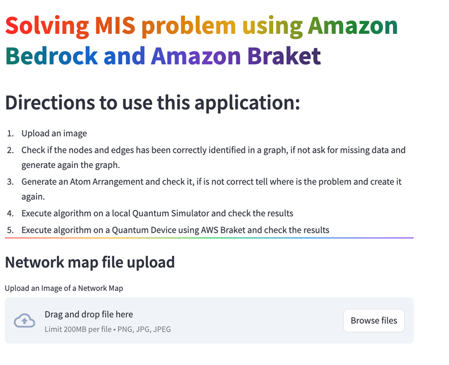

Figure 6: Landing page of the generative-AI application

Upload a file containing a graph with red circles and red lines. The image should follow this specific format for optimal processing. If you prefer to use a different graph representation, then you can modify the PROMPT_LLM_DIRECT_INVOCATION_IMAGE_PROCESSING parameter in the Prompts.py file.

After uploading your file, you should see a button that processes the image and generates a network graph visualization, as shown in the following figure.

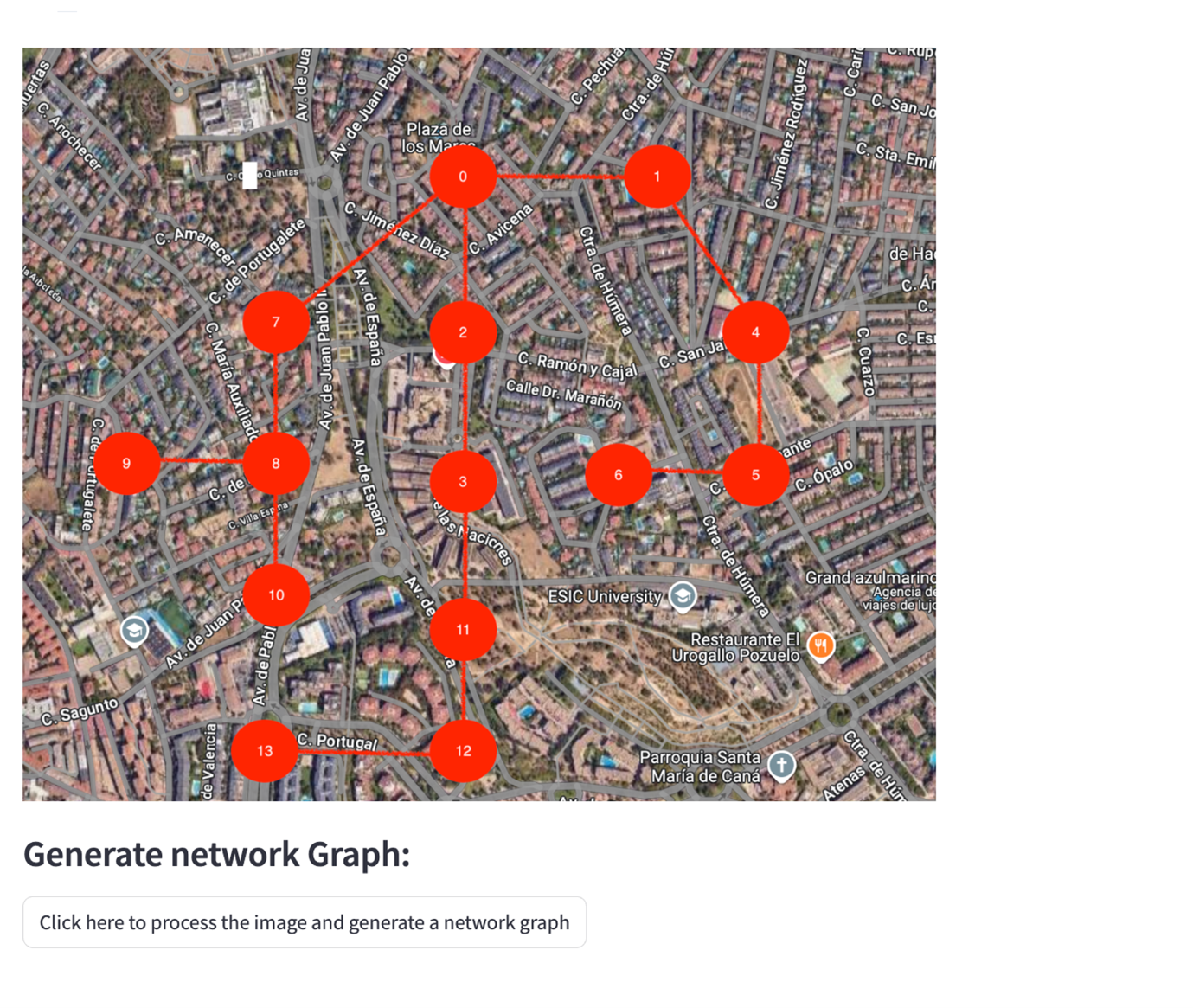Figure 7: Sample image of the reference RAN architecture

When you choose it, an Amazon Bedrock Agent processes your request through the following steps:

Image analysis: The Agent analyzes the uploaded image to identify nodes and edges within the graph structure.
Code generation and execution: Using the Agent’s code interpretation capabilities, it automatically generates and executes Python code to plot a graph diagram representing the network contained in the image.

The Agent uses the code interpretation feature of Amazon Bedrock to seamlessly handle this transformation from image to a Python graph and then to generate a graph file.

The resulting visualization appears in the web UI as shown in the following figure.

Figure 8: Initial (incorrect) network topology that can be modified using natural language

Working with Large Language Models (LLMs) presents unique challenges, such as potential hallucinations or inaccuracies in interpretation. In this example, the complexity of the input image—containing background text and road patterns—affects the model’s accuracy, resulting in an incorrect connection being generated between nodes 6 and 3.

However, thanks to the Agent’s ability to maintain context throughout the session, you can easily address these inaccuracies using natural language commands. The Agent maintains the conversation context, allowing you to do the following:

Identify incorrect connections
Request specific corrections
Refine the graph representation

This interactive correction capability demonstrates the flexibility of Amazon Bedrock Agents in handling real-world scenarios where initial interpretations may need adjustment.

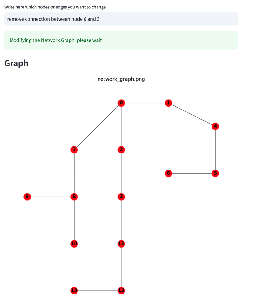
Figure 9: Generative-AI corrected version of the initial topology, modified using natural language

The image analysis and graph creation capabilities demonstrated by this Amazon Bedrock Agent open up exciting possibilities for advanced use cases. For example, you could do the following: analyze complex images to extract structured graph data, transform visual information into graph databases, and seamlessly integrate with services such as Amazon Neptune for further graph processing and analysis.

Although this post doesn’t delve into these advanced scenarios, we encourage readers to explore how these capabilities might enhance their own graph-based workflows and data processing pipelines. Combining the power of Amazon Bedrock Agents with other AWS services allows you to build sophisticated, AI-driven solutions that bridge the gap between visual and structured data.

The next step demonstrates how to create an Atom Arrangement visualization of your graph. Choosing the designated button triggers an Amazon Bedrock Agent to do the following:

Access the graph information stored in the session context
Process the updated data (such as any corrections you’ve provided)
Generate an Atom Arrangement visualization

The Agent uses the maintained session context to make sure that any modifications or refinements you’ve made to the graph structure are reflected in the final visualization, as shown in the following figure.

The Atom Arrangement grid is based on an arbitrary dimension-less unit distance that is mapped to a physical distance of 7mm, as shown later on.

Figure 10: One possible Atom Arrangement, corresponding to the reference network topology

We have obtained this structure called Atom Arrangement, a term that we mentioned a few times so far. But why an Atom Arrangement? In the following sections we explore some key concepts that are fundamental to understanding this solution.

Amazon Braket

Amazon Braket is a fully managed AWS service that helps researchers, scientists, and developers get started with quantum computing. It offers access to devices that consist of either an actual Quantum Processing Unit (QPU) or simulators that you can call to run a quantum task, for example, to solve the problem stated previously.

QPU types

Multiple companies and research groups are investigating different technologies to build a quantum computer, such as gate-based, quantum annealers and analog QPU, because different computation models excels at specific tasks. Amazon Braket offers a broad choice of QPUs from leading providers such as IonQ, IQM, and Rigetti, all based on the universal gate-based, and QuEra based on analog programming.

A gate-based QPU runs a quantum circuit, consisting of a series of unitary operations (called quantum gates) on the state of a register of qubits. This produces a stochastic measurement outcome at the end in the form of a bit string. This is a similar concept of traditional gate operations such as NOT, AND, and OR that can be combined to create an arbitrary logical circuit. However, quantum gates are fundamentally different from electronic gates, because they use quantum principles such as superposition and entanglement. This computation model is called digital quantum computing.

Analog quantum processors offer a versatile approach with applications in quantum simulation, optimization, and more. They can encode optimization problems in a more efficient way as compared to gate-based approach. On the other hand, they are not universal, because they can’t encode every possible problem.

In this post, we chose to use the analog quantum computer available in Amazon Braket: QuEra Aquila QPU. We chose this because it is a natural fit to solve the MIS/MVC optimization problem stated previously, and because it provides the largest number of qubits (256) available among QPUs accessible through Amazon Braket.

QuEra Aquila QPU can be programmed to solve optimization problems using three components that you can define as if you were in a traditional program where you encode problem and resolution in a programming language. In this case the QPU Program consists of an Atom Arrangement and two time varying functions called Global Rabi Frequency and Global Detuning.

In the following sections we describe those three elements of the QuEra Aquila QPU program.

QuEra Aquila QPU Program element: Atom Arrangement

For our problem, we use Atom Arrangement to encode the RAN topology in the QPU. Atom Arrangement consists of positioning atoms with x,y coordinates in a 2D grid. Each atom represents a base station (nodes of the graph) and connections between nodes (edges of the graph) are encoded with the distance among atoms: atoms closer than a specific distance called the Blockade Radius (we deep dive later in the post) are connected, and atoms at a higher distance than the Blockade Radius are not connected. This way of encoding graphs is called unit disk graph. In other words, in a unit disk graph, connections are functions of the nodes’ physical distance, while in a general graph there is not even the concept of physical distance among nodes.

The following figure shows an example of unit disk graph, where edges exist between nodes only if they are closer to each other than a fixed distance. In the QuEra Aquila QPU this is the Blockade Radius.

Figure 11: Example of a Unit Disk Graph: nodes are connected by edges only when they are within a fixed distance threshold of each other

Positioning atoms in the 2D area of the QPU allows you to create a great variety of graph topology. For example observe the following figure.

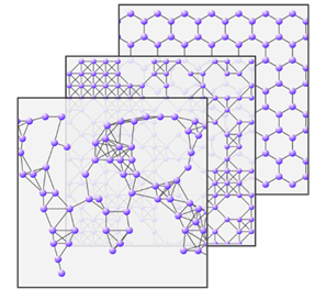Figure 12: Illustration of diverse Atom Arrangements showing the versatilitys of the Aqulia QPU)

The 2D area is a 76 μm x 75 μm size where you can position atoms (Rubidium-87 atom) using lasers as optical tweezers, based on the provided Atom Arrangement.

Before using the QPU to solve our problem, we must map the RAN topology to the QPU Atom Arrangement that is not a direct task. For this reason we have created the application based on a code generation enabled generative-AI agent that we have used in the previous section.

As a reminder, it assisted us in the following tasks:

Understanding the RAN topology from a map image.
Creating a graph where the nodes are the base stations and the edges are the existing connections among base stations.
Mapping the graph to the QPU Atom Arrangement, positioning the atoms so that connected nodes are represented by atoms closer than the Blockade Radius and unconnected nodes are represented by atoms farther than the Blockade Radius.

The outcomes of Steps 2 and 3 are reported hereafter just to recall what we obtained using the generative-AI assistant. Different valid Atom Arrangements can be generated by the application.

Figure 13: Mapping of the reference network topology to the corresponding Atom Arrangement.

With the Atom Arrangement in place, we can now execute our quantum algorithm through two distinct paths:

1. Local device simulation

First, we validate the algorithm using a local quantum circuit simulator.

2. Physical QPU execution

Then, we run the same algorithm on a real QuEra Aquila QPU device.

The Amazon Bedrock Agent processes the results from both execution paths by doing the following:

Analyzing the response from the quantum execution functions
Interpreting the quantum measurements
Visualizing the MIS solution
Rendering the results with color-coded nodes to distinguish set membership

The following figures demonstrate the results from the QPU simulator. Red identifies the MIS, while blue identifies the MVC.

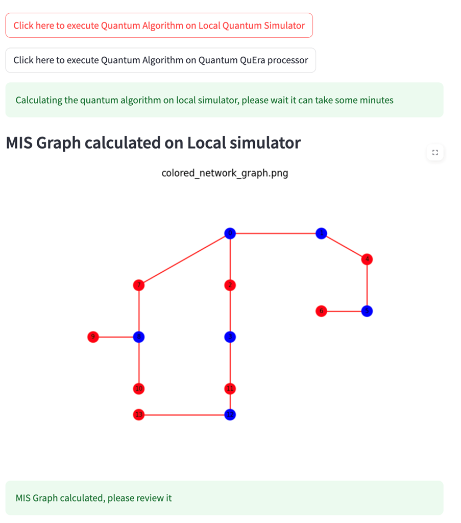Figure 14: Result from the local simulator: Red nodes represent the MIS of the reference RAN

Important: The execution of quantum algorithms on physical hardware depends on the availability of the QuEra Aquila QPU. If the device is unavailable, then your task is queued for execution on the next available time slot.

To check the current status and details of the QuEra Aquila QPU:

1. Navigate to the AWS Management Console.

2. Open the Amazon Braket service.

3. Choose Devices from the navigation pane.

4. Locate the QuEra Aquila QPU in the device list.

The following figure shows the device details page, where you can monitor the following:

Current device status
Queue information
Device specifications
Available time slots

This transparency in device availability helps you plan your quantum workloads effectively and understand potential execution delays.

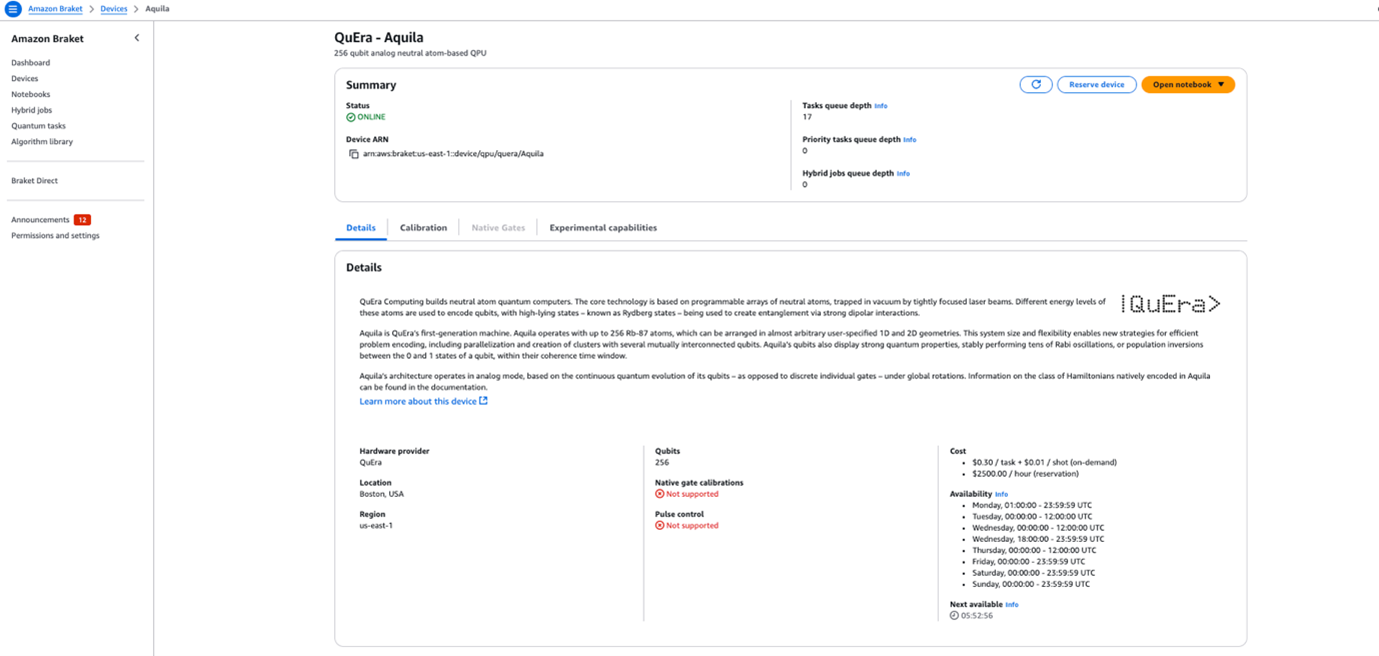Figure 15: Aqulia QPU weekly availability slots

When the QuEra Aquila QPU shows an ONLINE status, the QPU is available according to the Availability Calendar.

For an optimal user experience, we recommend executing the following part when the Tasks queue depth value is 0, so that you can get results in a short period of time (a few minutes). In case the queue is larger than 10, you could experience a timeout in the generative-AI application.

To initiate the QPU execution:

Verify that the QPU status is ONLINE in the Amazon Braket console.
Verify that the QPU is available according to the Availability Calendar.
Check that the queue length is within acceptable limits for you
Choose Execute on QPU in the user interface.

Figure 16: Generative-AI application button to execute the quantum algorithm on the QuEra Aquila QPU

The task status changes to RUNNING, then you should have the results on the screen. You can also track task status in the Amazon Braket console by navigating to the Quantum Task screen:

Figure 17: Amazon Braket console to check the Quantum Task status

But what is happening when executing the task in the QPU? After the Atom Arrangement was defined it was sent as an input parameter to a Python function. The function uses Amazon Braket SDK to interact with the QPU. But how were the atoms “excited” and how was the problem solved? We can dive deep into some detailed QuEra Aquila QPU program elements.

The overall process can be summarized as follows:

Positioning the atoms according to the Atom Arrangements to represent the graph.
Exciting the system with Global Rabi Frequency and Global Detuning functions.
Measuring the final status of the Atoms and mapping them to MIS or MVC nodes.

We have already discussed Atom Arrangements. Before proceeding with the second step, exciting the system, we can go into how a qubit is implemented in QuEra Aquila QPU to solve our problem.

Qubit in QuEra Aquila QPU

Each atom we positioned in the Atom Arrangement is a Rubidium-87 (Rb-87) atom, and we use its valence electron state to encode a single qubit. The valence electron is the most external electron of the atom. In the following figure you can see a representation of the ground state of the electron |g> and the Rydberg status |r>. The ground state orbit |g> is actually orders of magnitude smaller than the Rydberg state orbit .The ground state of the electron |g> represents the |0> state and the Rydberg status |r> represents the |1> state. The ket representation |status> is used in Quantum Mechanics to represent a quantum state. The |0> state represents the lowest possible energy of the electron while the |1> state is a very high energy state.

Figure 18: Valence electron status of the Rubidium-87 atom is used to encode a qubit

When we initially place the atoms in the Atom Arrangement, they are all at the minimum energy state |g> (the |0> state), the ground state. To move the system to the desired state, we must “excite” the atoms and reach a new final state that represents the solution to the problem where all (and only those) atoms not connected are in the |r> state. This is where we apply the QuEra Aquila QPU Program Elements called Global Rabi Frequency and Global Detuning functions.

QuEra Aquila QPU Program Elements: Global Rabi Frequency and Global Detuning functions

To excite the atoms, the QPU offers laser pulses with controlled intensity and frequency that drive the atoms’ states between |g> (low energy) and |r> (high energy) states or a combination of those states, called superpositions. The laser pulses, also known as control fields, are called Global Rabi Frequency and the Global Detuning function.

The Global Rabi Frequency function controls the laser intensity, while the Global Detuning function adjusts the frequency of the laser around a resonant frequency f₀ that is a specific property of the atom (more precisely of the |g> and |r> states we discussed). At that specific f₀ frequency the atom state oscillates between the |g> and |r> states.

In summary, with proper design of the Global Rabi Frequency and Global Detuning function, we can control the time evolution of the states of the atoms: high energy state, low energy state, or a superposition of those.

However, our system consists of several atoms that we accurately placed according to the Atom Arrangement. The atoms’ states are not only controlled by the described control fields, but also affected by the reciprocal distance of the atoms: this phenomenon is called Rydberg Blockade. The closer the atoms are together, then the higher the energy is needed to excite both atoms. If they are “close enough”, then the driving field that could excite the isolated atom can’t excite both atoms, so they can’t be both in the |r> states.

A peculiar distance in this context is the Rydberg Radius, shown in the following figure. On the left two atoms are farther apart than the Blockade Radius, and they can both be excited at the |r> state, while on the right the two atoms are closer than the Blockade Radius and only one can reach the |r> state.

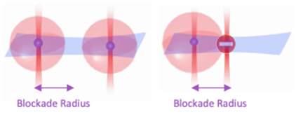
Figure 19: Illustration of the Rydberg Blockade phenomenon

Thanks to this property, it is appropriate to map the |r> state atoms to independent nodes belonging to the MIS. The final desired state of the atom arrangement is that all atoms that are not close to each other are in the |r> state. This state corresponds to the MIS of the graph. But how can we reach this state?

We can obtain this by slowly modifying the system from the initial state to the final desired state. The Adiabatic Theorem states, at a high level, that under slow enough modifications of the parameters of a quantum system, its ground state can be smoothly transformed while remaining in the lowest energy state. In other words we move from an all |g> system, with no external exciting energy, to a final desired state that is still in its lowest energy state of the new parameter setting. We can control the system evolution with the Global Rabi Frequency and the Global Detuning function.

In other words, our approach uses the physical properties of the system to find the minimum energy state, rather than relying on conventional optimization algorithms. The process works as follows:

In the initial state, all atoms are at their minimum energy level, denoted as |g⟩.
Then, we carefully design excitation waveforms that transition the system to a new state that corresponds to the problem we aim to solve (in this case, the MIS problem).
This transition must occur gradually, allowing the system to evolve slowly from its initial minimum to the final minimum through a series of quasi-stationary intermediate states.

Maintaining this slow evolution makes sure that the system follows a natural path through successive minimum energy configurations, ultimately reaching the solution state.

The design of the driving field, namely the Global Rabi Frequency and the Global Detuning function, given the Atom Arrangement is critical to obtain the desired final MIS state. For this post, we consider the functions available in the QuEra training, because they can move slowly the system from initial all ground |g> state to a final one where all atoms are in the |r> state, provided that they are farther than the blockade radius. The rules we have to respect to obtain the desired final status are as follows:

RULE 1: The Global Detuning max value must be about 2.7 times the max Global Rabi Frequency.

RULE 2: The Rydberg Radius must be about 1.2 times the minimum atoms distance.

RULE 3: The Global Detuning function must start from a large negative, end at a large positive, and change gradually in between.

RULE 4: The Global Rabi frequency value must be high when the Global Detuning crosses zero.

Rule 1 and 2 are not universal, but adopted from QuEra training. Rules 3 and 4 reflect the requirements of the Adiabatic Theorem.

With this in mind, we can analyze the most important features of the values assumed by the Global Rabi Frequency and Global Detuning function.

Figure 20: Waveforms of the Global Rabi Frequency and the Global Detuning function

Initial and final value of the Global Rabi Frequency must be 0 as necessitated by the QPU.
The maximum value of the Global Rabi Frequency is the maximum allowed value by the QPU (15.8×10⁶ rad/sec). The higher the Global Rabi Frequency the smaller the Blockade Radius. Specifically, this frequency corresponds to a 8.37 μm Blockade Radius. We choose 7 μm as the minimum atom distance in the Atom Arrangement, so that the Blockade Radius is about 1.2 times the minimum atom distance (RULE 2).
The maximum value of Global Detuning is equal to 2.7 times (RULE 1) the maximum Global Rabi Frequency (equal to 42.7×10⁶ rad/sec)
The initial value of Global Detuning must be large and negative to make sure that in the initial state all atoms are in the ground state |g>. We adopt the Maximum as in point 3 but with a value with a negative sign (equal to -42.7×10⁶ rad/sec).
The Global Rabi Frequency and Global Detuning function are changing “slowly” and “smoothly” in a linear way, to use the Adiabatic Theorem.

The time duration of the waves is 4 μs, and after that the final status of the atoms is measured as either |r> or |g>. Atoms in the |r> state correspond to the nodes in the MIS, while atoms in the |g> state correspond to nodes in the MVC.

Because the system is affected by noise, such as laser noise, atom motion, state decoherence, and the measurement process (see section 1.4) we must perform the same process several times. Furthermore, according to the AWS reference notebook, we must consider as a solution the most frequently measured configurations of |r> and |g> states. Each execution of the process is called a “shot”. All results of the shots are included in the QPU Program. In the best practices (see page 2), there is a trade-off between shot noise and speed/cost: 100 shots is a good middle ground between noise effect and speed/cost, with up to 1000 shots if you are interested in results with a low-probability outcome.

More resources to deep dive into the QuEra Aquila QPU and its usage to solve the MIS problem are available in this GitHub link.

A deep dive paper with a methodology to solve a wide range of problems using QuEra Aquila QPU can be found here.

Finally, a hands-on course about QuEra Aquila QPU can be found here.

Conclusion and benefits of the quantum approach

As we’ve demonstrated throughout this post, the integration of Amazon Braket and Amazon Bedrock allow for the studying of the prospects of quantum algorithms for optimization problems that telecom companies face.

For example, using quantum computing capabilities through Amazon Braket and enhancing solution workflows with AI-powered assistance from Amazon Bedrock allow telecom operators to optimize network infrastructure.

Our case study on backhaul network upgrades showcases just one of many potential applications where a quantum algorithm is applied to minimize fiber infrastructure costs while maximizing network performance.

Although we used a streamlined educational example to illustrate the concepts, the approach potentially scales to much larger, real-world scenarios, because quantum computing is evolving to accelerate the development of real world quantum computing applications.

As quantum computing technology continues to mature, telecom companies that begin experimenting with these solutions today should be well-positioned to transform their operations and gain competitive advantages in the future. We encourage you to explore the sample code provided, experiment with different network topologies, and join the growing community of quantum computing innovators on AWS.

Stay tuned for more exciting developments in the intersection of quantum computing and telecommunications!

AWS for Industries