Use Graph Machine Learning to detect fraud with Amazon Neptune Analytics and GraphStorm

Every year, businesses and consumers lose billions of dollars to fraud, with consumers reporting $12.5 billion lost to fraud in 2024, a 25% increase year over year. People who commit fraud often work together in organized fraud networks, running many different schemes that companies struggle to detect and stop. In this post, we discuss how to use Amazon Neptune Analytics, a memory-optimized graph database engine for analytics, and GraphStorm, a scalable open source graph machine learning (ML) library, to build a fraud analysis pipeline with AWS services.

Advantages of graph machine learning

Large Language Models (LLMs) excel at language tasks, while traditional machine learning works well with independent, structured data. However, many real-world problems—such as fraud detection— involve highly interconnected entities where relationships are as important as the entities themselves.
Graph machine learning (Graph ML) offers unique capabilities that go beyond both approaches, by explicitly capturing multi-hop relationships and structural patterns. Using GraphStorm, customers can use Graph Neural Networks (GNNs) to learn from these relationships across large-scale graphs. For example, graph analytics with graph ML can help surface:

• Indirect or hidden connections between users, accounts, and transactions
• Repeating network motifs such as transaction loops or degree anomalies
• Community structures that indicate coordinated behavior or emerging fraud rings

These structural signals are often missed by tabular models or LLMs that don’t analyze relationships directly. Moreover, graphs are dynamic, with new entities and links emerging constantly. GraphStorm supports cost-efficient incremental retraining on evolving graph data, enabling customers to update models efficiently—without the costly retraining or fine-tuning typically required for LLMs.
In short, Graph ML offers a powerful, complementary approach—especially in domains like fraud detection—where the structure and evolution of relationships provide critical signals. Customers like Careem have entrusted Amazon Neptune and graph ML to build their fraud detection system.

Overview of Neptune Analytics and the GraphStorm ML library

Neptune Analytics is a high-performance analytics engine for graphs, designed to provide insights and execute queries on massive, billion-scale graphs in seconds. It supports a library of graph analytics algorithms like community detection and supports storing node embeddings and performing efficient vector search for node similarity.

GraphStorm is an open-source graph ML library built for enterprise-scale applications that welcomes both beginners and experts in graph machine learning. With native AWS integration, GraphStorm simplifies the ML workflow through its high-level command line interface (CLI), enabling rapid, no-code model training. For developers who need deeper customization capabilities, GraphStorm’s Python API provides the flexibility to adapt models to meet specific use cases.

Solution overview

Fraud analysts need tools that allow them to focus their limited resources on the most suspicious users and activities, and they need to be able to query potentially massive graphs with complex queries in an interactive manner as they analyze new types of fraud.

A fraud analyst can enrich their original graph with representations and predicted risk scores from graph ML models trained in GraphStorm and then apply graph analysis methods like community detection interactively in Neptune Analytics. This creates a learning loop where, as new fraud behaviors arise, the predictions of the model can help fraud analysts uncover them, which in turn can assist the model in making better predictions in the future.

The steps to enrich a Neptune Analytics graph with GraphStorm embeddings and predictions are:

1. Export data from Neptune Analytics to Amazon Simple Storage Service (Amazon S3).
2. Describe the graph structure with a configuration file that GraphStorm uses as input.
3. Train a graph ML model and produce predictions and embeddings using GraphStorm on Amazon SageMaker AI.
4. Enrich graph data and import back into Neptune Analytics.
5. Perform fraud analysis using a Neptune Analytics graph notebook.

We illustrate the architecture and data flow in Figure 1.

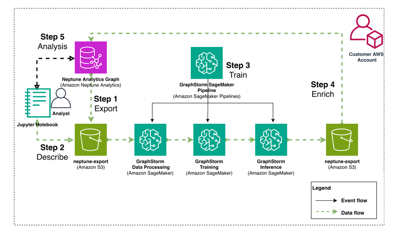
Figure 1: Architecture diagram showing data flow between Neptune Analytics and GraphStorm

Prerequisites

To run this example, you need the following:

• An AWS account.
• An S3 bucket for intermediate data
• One or more IAM roles to run the examples, with permissions to
  • Read and write to an S3 bucket.
  • Permissions to deploy and execute SageMaker AI pipelines.
  • Permissions to interact with a Neptune Analytics graph instance. Specifically, you need to have permission to create a new graph, start an import task and monitor its execution, and be able to delete the graph during the cleanup step.
• A SageMaker execution role with permissions to read and write to your S3 bucket.
• An Amazon SageMaker Studio domain. For instructions, refer to Use quick setup for Amazon SageMaker AI.

For instructions to create and use SageMaker AI roles, refer to Amazon SageMaker Role Manager, and for more information about Neptune Analytics identity and access management, see Identity and access management for Neptune Analytics.

Note: This example uses various AWS services including Amazon Neptune Analytics, Amazon SageMaker AI, and Amazon S3, and you will be responsible for any costs incurred while running these services. While AWS offers a Free Tier for some services, we recommend monitoring your usage carefully and reviewing the pricing pages for Neptune Analytics, SageMaker AI, and S3 before proceeding. Remember to follow the cleanup instructions at the end of this post to avoid ongoing charges.

Dataset overview

In this post, we use the IEEE CIS fraud dataset, an anonymized dataset that contains 500,000 transactions between users, a small percentage of which (around 3.5%) are identified as fraudulent. The goal is to develop a model that can correctly identify fraudulent transactions.

Each transaction is described by more than 300 categorical and numerical features, some of which can be used to form a transaction graph. For example, we use the properties named card1-card6 to create payment card node types, along with product code, addresses, and purchaser or recipient email domain node types. Every transaction includes a label named isFraud that marks the transaction as fraudulent or not.

The data is initially stored in two tabular files, which you convert to a graph representation that matches the format of a Neptune Analytics export task. This way, you can directly start with the learning pipeline steps. The Neptune samples repository you cloned above include examples of how to import and export graph data into and from a Neptune Analytics graph. The following diagram demonstrates a snippet from the graph structure, showing a transaction node connected to location, card type, and email nodes.

Figure 2: Example graph structure showing a transaction node connected to location, card type and email nodes.

Environment setup

To follow along with the post you can clone the amazon-neptune-samples repository and prepare your environment using:

# Clone graphstorm repository
git clone https://github.com/awslabs/graphstorm.git $HOME/graphstorm
# Clone example repository and navigate to example code
git clone https://github.com/aws-samples/amazon-neptune-samples.git 
cd amazon-neptune-samples/neptune-analytics-graphstorm-fraud-detection
# Set up python environment
python -m venv .venv
# Activate the virtualenv (bash example)
source .venv/bin/activate
pip install -r requirements.txt
# Launch the first notebook
jupyter-lab 0-Data-Preparation.ipynb

Create a Neptune Analytics graph

In 0-Data-Preparation.ipynb you start by creating a Neptune Graph in the background while you work through the rest of the notebooks. You will use this graph to import the graph data after you have enriched them with GNN embeddings and predictions.

import boto3
neptune_graph = boto3.client("neptune-graph")
# You need to choose node embedding size at graph creation time
EMBEDDING_SIZE = 128
GRAPH_NAME = "ieee-cis-fraud-detection"
# Create a Neptune Analytics graph
create_response = neptune_graph.create_graph(
    graphName=GRAPH_NAME,
    deletionProtection=False,
    publicConnectivity=True,
    vectorSearchConfiguration={"dimension": EMBEDDING_SIZE},
    replicaCount=0,
    provisionedMemory=16,
)
# Make a note of the graph ID for later use
GRAPH_ID = create_response["id"]

Create input for GraphStorm

In 0-Data-Preparation.ipynb you create data that are formatted the same as a Neptune Analytics export.

from graph_data_preprocessor_neptune import create_neptune_data
BUCKET=<your-s3-bucket>
PROCESSED_PREFIX = f"s3://{BUCKET}/neptune-input/{GRAPH_NAME}"
INPUT_S3 = (
    "s3://sagemaker-solutions-us-west-2/Fraud-detection-in-financial-networks/data"
)
ID_COLS = "card1,card2,card3,card4,card5,card6,ProductCD,addr1,addr2,P_emaildomain,R_emaildomain"
CAT_COLS = "M1,M2,M3,M4,M5,M6,M7,M8,M9"
create_neptune_data(
    output_prefix=PROCESSED_PREFIX,
    data_prefix=INPUT_S3,
    id_cols=ID_COLS,
    cat_cols=CAT_COLS,
)

The script creates the graph data under <PROCESSED_PREFIX>/graph_data and separate train/validation/test splits of the data under <PROCESSED_PREFIX>/graph_data/data_splits.

In notebook 0-Data-Preparation.ipynb we include an example of how to export an existing Neptune Analytics graph.

Extract graph ML task information for GraphStorm training

After you have exported your graph into a tabular representation of edge lists and node property files, GraphStorm needs a JSON file that describes your graph as a starting point. The JSON file describes how the files correspond to the graph schema, and the learning task to prepare the data for. GraphStorm can perform feature transformations and will apply the necessary data manipulation to make your dataset ready for distributed training.

By querying the Neptune Analytics service, you can programmatically generate such a JSON file, and we include a small utility with this post that extracts information from the files and queries the Neptune Analytics service to generate the GraphStorm configuration file that describes the data. In notebook 0-Data-Preparation.ipynb run:

import os.path as osp
from neptune_gs.create_gconstruct import create_graphstorm_config

EXPORTED_GRAPH_S3 = osp.join(PROCESSED_PREFIX, "graph_data")
gs_config = create_graphstorm_config(
    EXPORTED_GRAPH_S3, # S3 path under which you exported the graph 
    graph_id=GRAPH_ID, # Neptune Analytics graph ID
    learning_task="classification", # The learning task you want to perform
    target_type="Transaction", # The node type we want to predict on
    label_column="isFraud:Int",  # The name of the label column in the data.
)

For this dataset, we apply a min-max transformation to all numerical features and treat all string features as categorical. You will need to adapt the logic for other datasets that don’t meet these criteria.

The create_graphstorm_config function returns a Python dictionary that you save as a JSON file under the same location as the exported graph data. You are now ready to begin training your graph ML model.

SageMaker pipeline deployment and GNN training using GraphStorm

Graph ML on massive graphs is usually an involved, multi-step process:

1. Convert nodes and edges to a binary distributed graph representation.
2. Set up a distributed cluster.
3. Train the model.
4. Run inference.

Prepare GraphStorm image and create SageMaker Notebook instance

To ease the process, GraphStorm includes helper scripts to help you deploy SageMaker pipelines that handle the MLOps and orchestration needed, so you can focus on model development and not worry about setting up and maintaining ML infrastructure.

GraphStorm uses SageMaker AI Bring-Your-Own-Container (BYOC). To run GraphStorm jobs on SageMaker AI, you need to build and push GraphStorm’s training and graph processing image. For instructions, see Setup GraphStorm SageMaker Docker Image.

To set up the images and notebook needed to run through this example, execute notebook 1-SageMaker-Setup.ipynb that builds and pushes the GraphStorm image, and prepares a SageMaker notebook instance you will use to query the enriched Neptune Analytics graph.

Deploy and execute GraphStorm SageMaker Pipeline

In notebook 2-Deploy-Execute-Pipeline.ipynb you deploy and execute a GraphStorm SageMaker Pipeline. To deploy the pipeline, you need to provide a training configuration file that describes the type of model you want to train. For this example, we include two configuration files, one for training and one for inference, and a helper script to deploy the SageMaker AI pipeline.

TRAIN_YAML = "ieee_cis_nc_training.yaml"
INFERENCE_YAML = "ieee_cis_nc_inference.yaml"
YAML_S3_PREFIX = f"s3://{BUCKET}/yaml/{GRAPH_NAME}"

To upload the files to S3 in notebook 2-Deploy-Execute-Pipeline.ipynb run the cell

!aws s3 cp $TRAIN_YAML $YAML_S3_PREFIX/$TRAIN_YAML
!aws s3 cp $INFERENCE_YAML $YAML_S3_PREFIX/$INFERENCE_YAML

You also need to provide an execution role that the SageMaker AI jobs will use during graph processing and training. In notebook 2-Deploy-Execute-Pipeline.ipynb run:

# Location where you cloned GraphStorm
GS_HOME=$HOME/graphstorm
SM_EXECUTION_ROLE=<sagemaker-execution-role >
PIPELINE_NAME="graphstorm-ieee-cis-fraud-detection"
GCONSTRUCT_CONFIG="ieee-cis-gconstruct-node-classification.json"
PIPELINE_NAME = f"{GRAPH_NAME}-graphstorm-pipeline-gconstruct"

!bash deploy_fraud_detection_pipeline.sh \
    --bucket-name $BUCKET \
    --config-filename $CONFIG_FILENAME \
    --execution-role $SM_EXECUTION_ROLE \
    --input-s3 $EXPORT_PREFIX \
    --pipeline-name $PIPELINE_NAME \
    --train-yaml-s3 "$YAML_S3_PREFIX/$TRAIN_YAML" \
    --inference-yaml-s3 "$YAML_S3_PREFIX/$INFERENCE_YAML" \
    --graphstorm-location $GS_HOME 

After you deploy the pipeline, you can navigate to SageMaker Studio, choose the domain and user profile you used to create the pipeline, and choose Open Studio.

In the navigation pane, choose Pipelines. There should be a pipeline named ieee-cis-fraud-detection-graphstorm-pipeline-gconstruct. Choose the pipeline, which will take you to the Executions tab for the pipeline. Choose the graph to view the pipeline steps and their execution status.

The following screenshot shows the GraphStorm fraud detection model pipeline once the execution is complete.

Figure 3: GraphStorm fraud detection model pipeline

The pipeline has set up the necessary steps to process the data, run distributed training, and run inference to generate predictions and embeddings for every transaction node. To execute the pipeline, use the following code:

# Set a specific subpath to have for the execution
import time
timestamp = f"{time.time():.0f}"
EXECUTION_SUBPATH = f"gs-pipeline-example-{timestamp}"

!python3 $GS_HOME/sagemaker/pipeline/execute_sm_pipeline.py \
--pipeline-name $PIPELINE_NAME \
--region us-east-1 \
--execution-subpath $EXECUTION_SUBPATH

The pipeline will take around 25 minutes to execute. When it’s complete, you will be ready to run offline evaluations on the model predictions and import them back into Neptune Analytics to run graph analytics, with the risk scores and a GNN embedding attached to each transaction.

Enrich Neptune Analytics exported graph data with GraphStorm predictions

The GraphStorm pipeline produces the model, embeddings, and prediction outputs on Amazon S3. You can use the artifacts that GraphStorm produced to enrich your existing graph data and perform offline evaluation before re-importing the data back into Neptune Analytics. In notebook 2-Deploy-Execute-Pipeline.ipynb you enrich your original graph data with embeddings and predictions on Amazon S3:

PIPELINE_OUT = f"s3://{BUCKET}/pipelines-output/{PIPELINE_NAME}/{EXECUTION_SUBPATH}"
EMB_S3 = f"{PIPELINE_OUT}/inference/embeddings/"
PRED_S3 = f"{PIPELINE_OUT}/inference/predictions/"

ENRICHED_S3 = f"s3://{BUCKET}/neptune-enriched/{GRAPH_NAME}"

attach_gs_data_to_na(
    input_s3=EXPORTED_GRAPH_S3,
    output_s3=ENRICHED_S3,
    embeddings_s3=EMB_S3,
    predictions_s3=PRED_S3,
    graph_id=GRAPH_ID,
)

The attach_gs_data_to_na function joins your original graph data for the Transaction node type with the generated embeddings based on node ID, and creates new node output files that include a new column named embeddings:Vector that Neptune Analytics will import into its vector index, and a column named pred:Float[] that includes the fraud risk score predicted by the model, a value from 0 to 1.0.

With the updated transaction data in hand, you can perform offline evaluations of the model performance. Following along notebook 3-Use-Embeddings-Locally.ipynb, load the original transactions and join them with the GraphStorm output to get predictions and embeddings for each Transaction

from os import path as osp
from neptune_gs.fs_handler import FileSystemHandler


# Get the GraphStorm embeddings and predictions
GRAPH_NAME = "ieee-cis-fraud-detection"
ENRICHED_S3 = f"s3://{BUCKET}/neptune-enriched/{GRAPH_NAME}/"
enriched_handler = FileSystemHandler(ENRICHED_S3)
transaction_files = enriched_handler.list_files(
pattern="Vertex_Transaction*")
transaction_emb_pred_df = enriched_handler.create_df_from_files(
    transaction_files)

Next load the original data and extract the true isFraud values, and join them with the model predictions

# Get the original data to gather the isFraud labels
original_handler = FileSystemHandler(EXPORT_PREFIX)
orig_transaction_files = original_handler.list_files(pattern="Vertex_Transaction*")
orig_transactions_df = original_handler.create_df_from_files(
    orig_transaction_files 
)
# Join original Transaction data with embeddings and predictions
transactions_with_fraud = transaction_emb_pred_df.set_index("~id").join(
    orig_transactions_df.set_index("~id")
)

Finally, get the ids of the transactions that were selected for your hold-out test set, to check the model’s performance on unseen data:

# Get predictions made for test data
NEPTUNE_INPUT_DATA = f"s3://{BUCKET}/neptune-input/{GRAPH_NAME}/data_splits"
test_ids = input_handler.create_df_from_files(
    [f"{NEPTUNE_INPUT_DATA}/test_ids.parquet"]
)
test_preds = test_ids.set_index("nid").join(
    transactions_with_fraud.set_index("~id"), how="left"
)
test_preds["pred:Float[]"] = test_preds["pred:Float[]"].astype("float")

Now you can plot the Receiver Operating Characteristic (ROC) curve to visualize the performance of the GNN model, with the performance shown in the following figure:

import matplotlib.pyplot as plt
from sklearn.metrics import RocCurveDisplay, PrecisionRecallDisplay

fig, [ax_roc, ax_pr] = plt.subplots(1, 2, figsize=(11, 5))
PrecisionRecallDisplay.from_predictions(
    y_true=test_preds["isFraud:Int"],
    y_pred=test_preds["pred:Float[]"],
    plot_chance_level=True,
    despine=True,
    ax=ax_pr,
)
RocCurveDisplay.from_predictions(
    y_true=test_preds["isFraud:Int"],
    y_pred=test_preds["pred:Float[]"],
    name="GNN",
    plot_chance_level=True,
    despine=True,
    ax=ax_roc,
)
ax_roc.set_title("Receiver Operating Characteristic (ROC) curves")
ax_pr.set_title("Precision-Recall curves")
ax_roc.grid(linestyle="--")
ax_pr.grid(linestyle="--")
plt.legend()
plt.show()

These graphs demonstrate the performance of the model at different threshold levels, providing a clear view into the model’s ability to separate fraudulent cases.

Figure 4: Performance curves showing ROC AUC of ~0.9 for the GNN model

The model can deal with the class imbalance, achieving an Area Under the ROC Curve of approximately 0.9, and maintain good precision/recall trade-offs at different threshold levels.

Now that you have verified the accuracy of the model, you can import the enriched graph back into Neptune Analytics and perform additional analysis with the capabilities that the service provides.

Import graph into Neptune Analytics

Before enriching the graph, you will first import the original graph data you created. For this, follow along notebook 4-Import-Embeddings-to-Neptune-Analytics.ipynb. You will need access to a Neptune Analytics import role.

NEPTUNE_IMPORT_ROLE = <your-neptune-analytics-import-role> 
neptune_graph = boto3.client("neptune-graph")
NEPTUNE_IMPORT_S3 = f"s3://{BUCKET}/neptune-input/{GRAPH_NAME}/graph_data"
# Start the import task
import_response = neptune_graph.start_import_task(
    graphIdentifier=GRAPH_ID,
    format="CSV",
    source=NEPTUNE_IMPORT_S3,
    roleArn=NEPTUNE_IMPORT_ROLE,
)

The data import should take 5-10 minutes to complete after which you will move to the SageMaker Notebook instance you created in notebook 1-SageMaker-Setup.ipynb to run OpenCypher queries against the Neptune Analytics graph.

Explore and analyze the transaction graph on Neptune Analytics to uncover and analyze fraudulent transactions

To run interactive analytics queries on your graph, you can use a graph notebook, which is a specialized Jupyter notebook that provides a number of Jupyter cell-magic commands that help with the execution of graph queries. You should have created such a notebook instance when running through notebook 1-SageMaker-Setup.ipynb. For instructions to create a graph notebook, see Creating a new Neptune Analytics notebook using the AWS Management Console.

When your notebook instance is available, you can open notebook 5-Explore-With-Neptune-Analytics.ipynb. In this notebook, you update the graph to include predictions and embeddings for the transaction nodes, and run Neptune Analytics queries on the graph that use the extra information provided by the predictions.

To begin, import the embeddings and predictions for the transaction nodes into your existing Neptune Analytics graph. First, set up the path to import data from:

# Run this cell as Python
BUCKET=<your-s3-bucket>
GRAPH_NAME="ieee-cis-fraud-detection"
ENRICHED_S3 = f"s3://{BUCKET}/neptune-enriched/{GRAPH_NAME}"

Then you can run neptune.load to load the predictions and embeddings:

%%oc
CALL neptune.load(
  {
    source: "${ENRICHED_S3}",
    region: "us-east-1",
    format: "csv"
  }
)

When the query finishes, your transaction nodes will include a new pred column that represents the risk score predicted by the model, and you will have access to Neptune Analytics vector similarity queries to compare transactions according to their GNN embeddings.

Combining graph analysis with GraphStorm predictions

As we mentioned in the introduction, fraudsters work in coordinated, hierarchical groups with strong connectivity between them. The Louvain method is a scalable community detection algorithm that can uncover community hierarchies on massive graphs. Neptune Analytics includes an efficient implementation of Louvain that you can use to annotate nodes in the graph with community identifiers. In a graph notebook, you can run the algorithm using the following code:

%%oc
CALL neptune.algo.louvain.mutate(
  {
    writeProperty: "louvainCommunity",
    maxLevels: 3,
    maxIterations: 10
  }
)
YIELD success
RETURN success

After Louvain has assigned a community to each node, you can use the extra information provided by the GNN model to uncover communities whose members have a higher risk on average.

Use the following query to rank communities that include at least 10 transactions by their average risk score. The query will store the list of risky communities into a Python variable using the --store-to argument to the %%oc magic command. Because this is an example dataset giving us access to all labels, we can also include the actual fraud rate in these communities to verify the predictions made by the model.

%%oc --store-to suspicious_communities

MATCH (t:Transaction)
WITH t.louvainCommunity as community_id,
     count(t) as tx_count,
     avg(t.pred) as avg_risk_score,
     avg(t.isFraud) as avg_fraud
WHERE tx_count > 10
RETURN community_id, tx_count, avg_risk_score, avg_fraud
ORDER BY avg_risk_score DESC LIMIT 10

To extract the riskiest community, you can run a Python snippet as follows:

# Extract the id of the community with the highest average risk
high_risk_community = suspicious_communities['results'][0]['community_id']

You can now use the results of this query to examine the community with the most risk on average. The following query will return suspicious transaction nodes in the community (with a risk score above 0.7), and 100 edges along with the nodes they connect to:

%%oc
MATCH (n) WHERE n.louvainCommunity = ${high_risk_community} 
MATCH p=(n)-[]->()
RETURN p
LIMIT 100

Figure 5: Transactions belonging to a suspicious community and their neighbors

In the returned neighborhood, you can see that all the suspicious transactions connect to a particular address value, addr1:441. This can be an indicator that this address warrants further investigation. The notebook we provided in this post includes even more advanced graph queries that you can run to combine graph analytics with GNN model predictions.

Use node embeddings to find transactions similar to high-risk transactions

The node embeddings that the GNN model has created contain semantic information about the characteristics of each transaction. Using the predicted risk scores, you can isolate high-risk transactions, then expand your search to similar transactions to find characteristics that join them. For example, you can get the top-k most similar transactions to each high-risk transaction using the following code:

%%oc --store-to high_risk_neighbors
MATCH (t:Transaction)
WHERE t.pred >= 0.8
WITH t LIMIT 5
CALL neptune.algo.vectors.topKByNode(t, {topK: 4})
YIELD node as similar_node, score
WHERE id(t) <> id(similar_node)
RETURN id(t), id(similar_node), score as distance, similar_node.pred, similar_node.isFraud

You can then investigate the connections between these transactions by retrieving the paths connecting them. First, extract the neighbor IDs in Python:

high_risk_neighbor_ids = [
    entry['id(similar_node)'] for entry in high_risk_neighbors['results']]

Then submit a new OpenCypher query to extract the sub-graph that contains the similar transactions and their neighbors:

%%oc
MATCH (n) WHERE id(n) = ${high_risk_neighbor_ids}
MATCH p=(n)-[]->()
RETURN p
LIMIT 100

The following figure shows a sample of transactions most similar to high-risk transactions and their neighbors.

Figure 6: A sample of transactions most similar to high-risk transactions and their neighborhood

In this example, the two transaction components are connected by three bridge nodes of types Address2, Card6, and Card4 (your results may vary). You can use the values of these nodes, which in this case are card4:visa, card6:credit, and addr2:87.0, and find other transactions that share the same characteristics as another way to uncover potentially risky transactions.

Future improvements and potential integrations

As an extension to this workflow, you can include a Neptune Database instance that makes it possible to serve online transactional graph queries, for example calculating the risk score for new incoming transactions based on their connections to existing nodes in the graph.

For an example of such a workflow that includes Neptune Database and Neptune Analytics, refer to Use Amazon Neptune Analytics to analyze relationships in your data faster, Part 1: Introducing Parquet and CSV import and export and Use Amazon Neptune Analytics to analyze relationships in your data faster, Part 2: Enhancing fraud detection with Parquet and CSV import and export.

Clean up

To stop accruing costs on your account, delete the Neptune Analytics graph you created for this post To do so, you can use the AWS Command Line Interface (AWS CLI) or the Neptune Analytics console. You can also remove any files you created on S3.

Conclusion

In this post, we demonstrated how to export data from Neptune Analytics, use GraphStorm on SageMaker AI to train a model on your exported graph data, and enrich your Neptune Analytics graph with GraphStorm node embeddings and predictions. This workflow empowers you to focus your graph analytics on nodes and node groups that are the most important to your business problem, in this case illustrated with a fraud analysis dataset.

To run though this example yourself, clone the Amazon Neptune Samples repository and run through the notebooks under the neptune-analytics-graphstorm-fraud-detection directory. To learn more about GraphStorm, refer to GraphStorm Documentation and Tutorials. To learn more about Neptune Analytics, see the Neptune Analytics User Guide.

About the authors