Optimize and troubleshoot database performance in Amazon Aurora PostgreSQL by analyzing execution plans using CloudWatch Database Insights

Amazon Web Services (AWS) offers a comprehensive suite of monitoring tools to increase visibility of performance and events for Amazon Relational Database Service (Amazon RDS) and Amazon Aurora databases. In this post, we demonstrate how you can use Amazon CloudWatch Database Insights to analyze your SQL execution plan to troubleshoot and optimize your SQL query performance in an Aurora PostgreSQL cluster.

PostgreSQL query optimizer and query access plans

The PostgreSQL query optimizer is a core component of the database engine and is responsible for determining the most efficient way to execute SQL queries. When a query is submitted, PostgreSQL doesn’t execute it directly, instead it generates multiple possible execution strategies and selects the optimal one based on cost estimation.

A query access plan is the step-by-step execution strategy chosen by the optimizer. It details how PostgreSQL will retrieve and process data, using techniques such as sequential scans, index scans, joins, and sorting operations. You can analyze query plans using the EXPLAIN command with options to understand execution paths.

Understanding the PostgreSQL query optimizer and query access plan is important for developers and database administrators to optimize database performance and optimize resource usage effectively. To learn more, see How PostgreSQL processes queries and how to analyze them.

Solution overview

In December 2024, AWS introduced CloudWatch Database Insights, a comprehensive database monitoring solution that supports Aurora (both PostgreSQL and MySQL variants) and Amazon RDS engines, including PostgreSQL, MySQL, MariaDB, SQL Server, and Oracle. This observability tool is specifically designed to help DevOps engineers, developers, and DBAs quickly identify and resolve database performance issues. By providing a unified view across database fleets, Cloudwatch Database Insights streamlines troubleshooting workflows and improves operational efficiency.

CloudWatch Database Insights has an Advanced mode and a Standard mode. The tool to analyze Aurora PostgreSQL execution plans is only available in Advanced mode. In the following sections, we show you how to enable the SQL execution plan analysis feature in your Aurora PostgreSQL clusters. We also guide you through troubleshooting query performance issues caused by plan changes and help you optimize query performance based on the query plan.

For this post, we use a typical e-commerce application schema that contains customer information, a product catalog, order details, and order line items. These elements are represented by corresponding tables – customers, products, orders, and order_items – which makes up the online retail database.

In the next sections, we show how you can analyze SQL execution plans for Aurora PostgreSQL-Compatible edition in CloudWatch Database Insights.

Prerequisites

To follow along with this post, some additional configuration is required. Refer the prerequisites in Analyzing execution plans with CloudWatch Database Insights for detailed information.

Analyze SQL execution plans

Let’s look at an example of a typical query executed against this application and how we can analyze the execution plans through CloudWatch Database Insights.

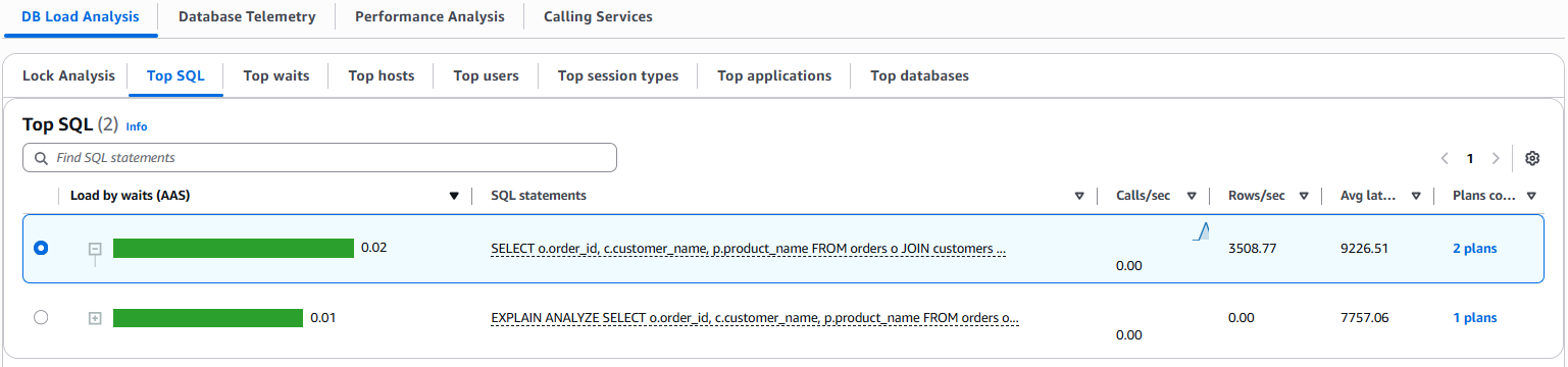
We begin our investigation by accessing CloudWatch Database Insights through the CloudWatch console. After navigating to Database Views, we locate our Aurora PostgreSQL DB instance and examine its performance metrics on the Top SQL tab.

The Plans Count column in the Top SQL table indicates the number of collected plans for each digest query. If needed, you can choose the settings icon to customize column visibility and ordering in the Top SQL table.

We then focus on the specific SQL statement executed by our e-commerce application. By selecting the digest query and reviewing its details on the SQL text tab, we can see the exact SQL statement being run. The Plans tab provide us with a detailed view of the query execution plans.

For comparative analysis, up to two plans can be selected simultaneously, as shown in the following screenshot.

Our side-by-side comparison of the two executions reveal a crucial difference: one plan used a sequential scan approach, whereas the other employed an index scan. This difference in access path selection provided valuable insights into query performance variations and resource utilization patterns.

Gather (cost=1000.00..266914.09 rows=95345 width=126) (actual time=0.264..307.518 rows=100799 loops=1)
Workers Planned: 2
Workers Launched: 2
-> Parallel Seq Scan on person (cost=0.00..256379.59 rows=39727 width=126) (actual time=0.023..367.948 rows=33600 loops=3)
Filter: (age = 40)
Rows Removed by Filter: 3299734

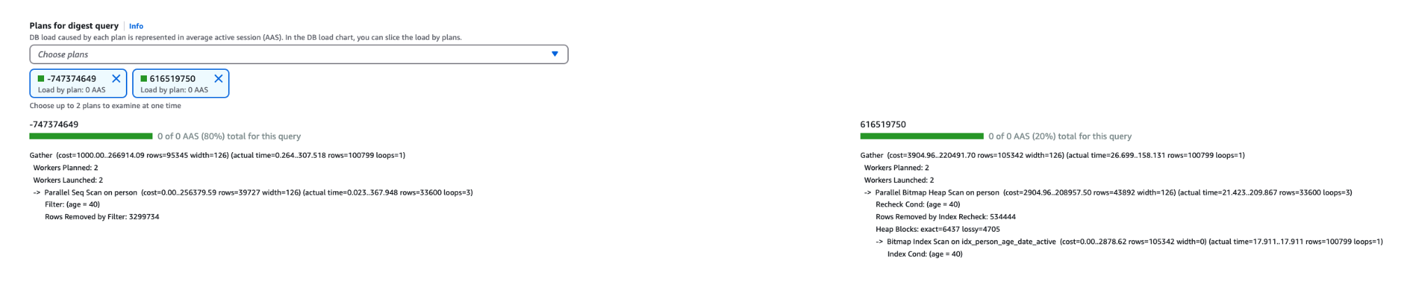
Second Execution plan 616519750:

Gather (cost=3904.96..220491.70 rows=105342 width=126) (actual time=26.699..158.131 rows=100799 loops=1)
Workers Planned: 2
Workers Launched: 2
-> Parallel Bitmap Heap Scan on person (cost=2904.96..208957.50 rows=43892 width=126) (actual time=21.423..209.867 rows=33600 loops=3)
Recheck Cond: (age = 40)
Rows Removed by Index Recheck: 534444
Heap Blocks: exact=6437 lossy=4705
-> Bitmap Index Scan on idx_person_age_date_active (cost=0.00..2878.62 rows=105342 width=0) (actual time=17.911..17.911 rows=100799 loops=1)
Index Cond: (age = 40)

Compare execution plans to troubleshoot performance degradation

When investigating SQL query performance degradation issues, DBAs and DBEs often rely on analyzing query execution plans. They look for changes in execution behavior that could impact performance, such as dropped indexes, inefficient join strategies, or suboptimal query patterns. However, manually comparing complex, nested execution plans across different time periods can be tedious and error-prone.For example, consider the following statement executed by our sample application. It retrieves order details along with associated customer and product information for orders placed after a specific date:

SELECT o.order_id, c.customer_name, p.product_name
FROM orders o
JOIN customers c ON c.customer_id = o.customer_id
JOIN order_items oi ON oi.order_id = o.order_id
JOIN products p ON p.product_id = oi.product_id
WHERE o.order_date > '2024-01-01';

To simulate a real-world scenario of accidental index deletion, we dropped some indexes on the orders and order_items tables, particularly those involved in join conditions, and updated the table statistics. These changes resulted in a suboptimal execution plan, causing the query to slow down dramatically and negatively impact overall application performance.

You can use CloudWatch Database Insights to compare execution plans for the same SQL statement over time. This simplifies troubleshooting by highlighting changes that might have led to performance degradation and helping teams quickly diagnose and resolve performance issues.The following screenshot shows the SQL query and its execution plan information from CloudWatch Database Insights. You can also copy or download the execution plans.

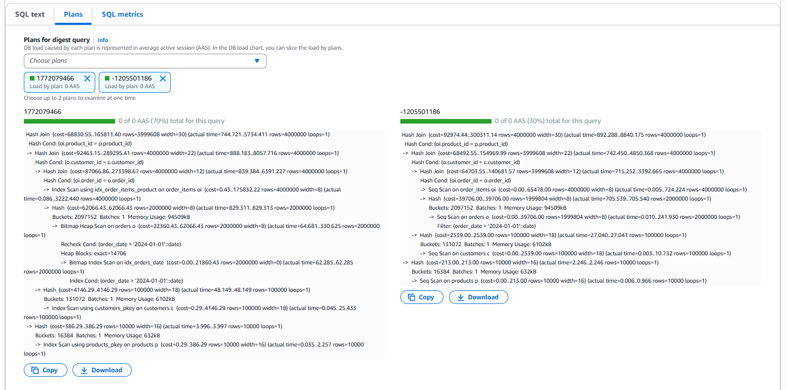
Following are the detail of execution plans as seen in above screenshots.

First Execution plan 1772079466

Hash Join (cost=68830.55..165811.40 rows=3999608 width=30) (actual time=744.721..5734.411 rows=4000000 loops=1)
Hash Cond: (oi.product_id = p.product_id)
-> Hash Join (cost=92463.15..289295.41 rows=4000000 width=22) (actual time=888.183..8057.716 rows=4000000 loops=1)
Hash Cond: (o.customer_id = c.customer_id)
-> Hash Join (cost=87066.86..273398.67 rows=4000000 width=12) (actual time=839.384..6391.227 rows=4000000 loops=1)
Hash Cond: (oi.order_id = o.order_id)
-> Index Scan using idx_order_items_product on order_items oi (cost=0.43..175832.22 rows=4000000 width=8) (actual time=0.086..3222.440 rows=4000000 loops=1)
-> Hash (cost=62066.43..62066.43 rows=2000000 width=8) (actual time=829.311..829.313 rows=2000000 loops=1)
Buckets: 2097152  Batches: 1  Memory Usage: 94509kB
-> Bitmap Heap Scan on orders o (cost=22360.43..62066.43 rows=2000000 width=8) (actual time=64.681..330.625 rows=2000000 loops=1)
Recheck Cond: (order_date > '2024-01-01'::date)
Heap Blocks: exact=14706
-> Bitmap Index Scan on idx_orders_date (cost=0.00..21860.43 rows=2000000 width=0) (actual time=62.285..62.285 rows=2000000 loops=1)
Index Cond: (order_date > '2024-01-01'::date)
-> Hash (cost=4146.29..4146.29 rows=100000 width=18) (actual time=48.149..48.149 rows=100000 loops=1)
Buckets: 131072  Batches: 1  Memory Usage: 6102kB
-> Index Scan using customers_pkey on customers c (cost=0.29..4146.29 rows=100000 width=18) (actual time=0.045..25.433 rows=100000 loops=1)
-> Hash (cost=386.29..386.29 rows=10000 width=16) (actual time=3.996..3.997 rows=10000 loops=1)
Buckets: 16384  Batches: 1  Memory Usage: 632kB
-> Index Scan using products_pkey on products p (cost=0.29..386.29 rows=10000 width=16) (actual time=0.035..2.257 rows=10000 loops=1)

Second Execution plan -1205501186

Hash Join (cost=92974.44..300311.14 rows=4000000 width=30) (actual time=892.288..8840.175 rows=4000000 loops=1)
Hash Cond: (oi.product_id = p.product_id)
-> Hash Join (cost=68492.55..154969.99 rows=3999608 width=22) (actual time=742.450..4850.368 rows=4000000 loops=1)
Hash Cond: (o.customer_id = c.customer_id)
-> Hash Join (cost=64703.55..140681.57 rows=3999608 width=12) (actual time=713.232..3392.665 rows=4000000 loops=1)
Hash Cond: (oi.order_id = o.order_id)
-> Seq Scan on order_items oi (cost=0.00..65478.00 rows=4000000 width=8) (actual time=0.005..724.224 rows=4000000 loops=1)
-> Hash (cost=39706.00..39706.00 rows=1999804 width=8) (actual time=705.539..705.540 rows=2000000 loops=1)
Buckets: 2097152  Batches: 1  Memory Usage: 94509kB
-> Seq Scan on orders o (cost=0.00..39706.00 rows=1999804 width=8) (actual time=0.010..241.930 rows=2000000 loops=1)
Filter: (order_date > '2024-01-01'::date)
-> Hash (cost=2539.00..2539.00 rows=100000 width=18) (actual time=29.162..29.162 rows=100000 loops=1)
Buckets: 131072  Batches: 1  Memory Usage: 6102kB
-> Seq Scan on customers c (cost=0.00..2539.00 rows=100000 width=18) (actual time=0.003..10.732 rows=100000 loops=1)
-> Hash (cost=213.00..213.00 rows=10000 width=16) (actual time=2.246..2.246 rows=10000 loops=1)
Buckets: 16384  Batches: 1  Memory Usage: 632kB
-> Seq Scan on products p (cost=0.00..213.00 rows=10000 width=16) (actual time=0.006..0.966 rows=10000 loops=1)

As seen in the execution plan details, there are significant differences between the two recorded execution plans for the same query, each with a direct impact on performance. The query execution plan on the lower left represents the original state, where appropriate indexes are in place, resulting in index scans on tables involved and a total query cost of 165811.40. In contrast, the execution plan on the lower right reflects the state after those indexes were accidentally dropped, leading to sequential scans on tables involved and a much higher total cost of 300311.14. This increase in cost clearly explains the performance degradation experienced after maintenance where the indexes got accidentally dropped.

Using the side-by-side execution plan comparison feature in CloudWatch Database Insights to determine the root cause of the performance degradation was simplified by automating what would typically require manual query plan extraction and comparison.

Analyze execution plans to optimize query performance

Analyzing a SQL query execution plan provides deep insights into how the database engine processes a query. By examining key elements such as join types, scan methods, Sorting techniques, estimated and actual row counts, and operator costs, you can identify inefficiencies and performance bottlenecks. These details help identify issues such as missing indexes, suboptimal join orders, outdated statistics, and misconfigured database parameters. You can then use this information to fine-tune queries and optimize performance.

For this example, consider the following statement executed by our e-commerce application that summarizes customer spending per order date, sorted from highest to lowest total amount spent. Database monitoring has identified degraded query execution times as the cause of the application slowdown and overall performance bottlenecks. We’ll demonstrate how to optimize query performance using CloudWatch Database Insights. As part of this process, we use EXPLAIN ANALYZE to examine the actual execution plan and identify opportunities for improvement.

SELECT c.customer_name, o.order_date, SUM(oi.quantity * p.price) AS total_spent
FROM customers c
JOIN orders o ON c.customer_id = o.customer_id
JOIN order_items oi ON o.order_id = oi.order_id
JOIN products p ON oi.product_id = p.product_id
GROUP BY c.customer_name, o.order_date
ORDER BY total_spent DESC;

The following screenshot shows the query execution plan in CloudWatch Database Insights.

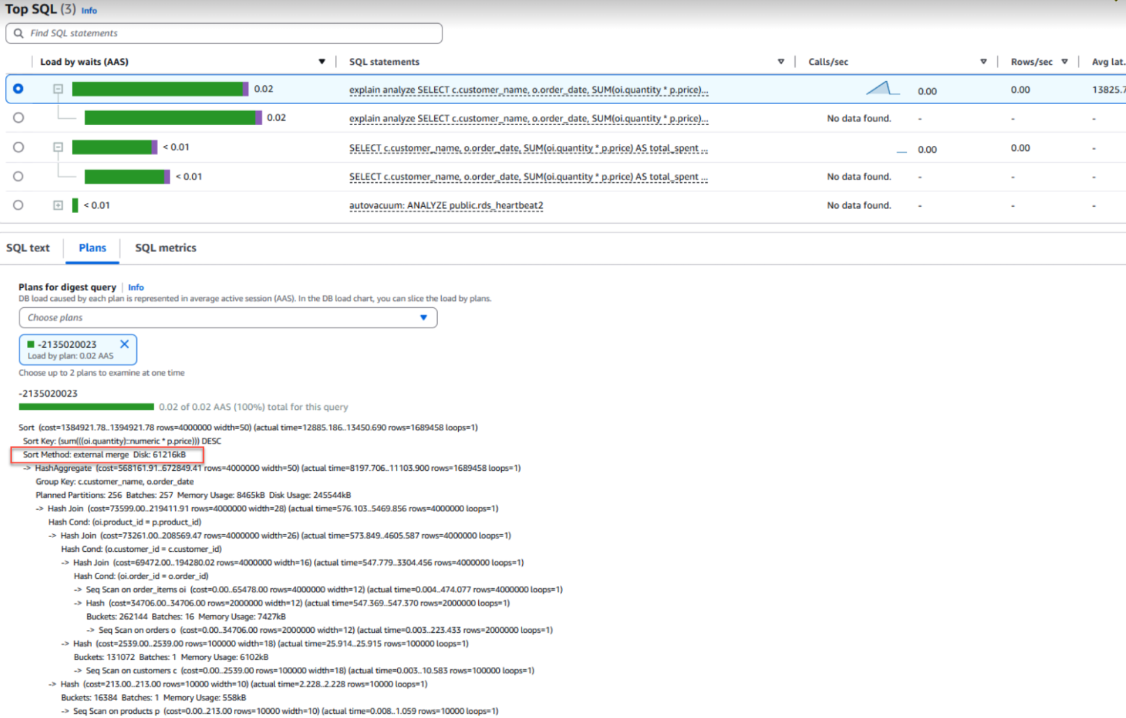
Here is the detail of execution plan as seen in above screenshot.

Execution plan -2135020023

Sort (cost=1384921.78..1394921.78 rows=4000000 width=50) (actual time=12885.186..13450.690 rows=1689458 loops=1)
Sort Key: (sum(((oi.quantity)::numeric * p.price))) DESC
Sort Method: external merge  Disk: 61216kB
-> HashAggregate (cost=568161.91..672849.41 rows=4000000 width=50) (actual time=8197.706..11103.900 rows=1689458 loops=1)
Group Key: c.customer_name, o.order_date
Planned Partitions: 256  Batches: 257  Memory Usage: 8465kB  Disk Usage: 245544kB
-> Hash Join (cost=73599.00..219411.91 rows=4000000 width=28) (actual time=576.103..5469.856 rows=4000000 loops=1)
Hash Cond: (oi.product_id = p.product_id)
-> Hash Join (cost=73261.00..208569.47 rows=4000000 width=26) (actual time=573.849..4605.587 rows=4000000 loops=1)
Hash Cond: (o.customer_id = c.customer_id)
-> Hash Join (cost=69472.00..194280.02 rows=4000000 width=16) (actual time=547.779..3304.456 rows=4000000 loops=1)
Hash Cond: (oi.order_id = o.order_id)
-> Seq Scan on order_items oi (cost=0.00..65478.00 rows=4000000 width=12) (actual time=0.004..474.077 rows=4000000 loops=1)
-> Hash (cost=34706.00..34706.00 rows=2000000 width=12) (actual time=547.369..547.370 rows=2000000 loops=1)
Buckets: 262144  Batches: 16  Memory Usage: 7427kB
-> Seq Scan on orders o (cost=0.00..34706.00 rows=2000000 width=12) (actual time=0.003..223.433 rows=2000000 loops=1)
-> Hash (cost=2539.00..2539.00 rows=100000 width=18) (actual time=25.914..25.915 rows=100000 loops=1)
Buckets: 131072  Batches: 1  Memory Usage: 6102kB
-> Seq Scan on customers c (cost=0.00..2539.00 rows=100000 width=18) (actual time=0.003..10.583 rows=100000 loops=1)
-> Hash (cost=213.00..213.00 rows=10000 width=10) (actual time=2.228..2.228 rows=10000 loops=1)
Buckets: 16384  Batches: 1  Memory Usage: 558kB
-> Seq Scan on products p (cost=0.00..213.00 rows=10000 width=10) (actual time=0.008..1.059 rows=10000 loops=1)

From the query execution plan, we notice a relevant clue: Sort Method: external merge Disk: 61216kB. This is a significant finding in our investigation. It indicates the database had to resort to disk-based sorting instead of keeping everything in memory. This external disk usage strongly suggests a performance bottleneck with the SQL statement.

Digging deeper into PostgreSQL’s parameter group configuration, we found that sorting operations are controlled by the work_mem parameter, currently set to its default value of 4 MB. While this setting was sufficient when our dataset was smaller, recent data growth has pushed memory requirements well beyond this limit. Our investigation shows that the query now requires approximately 61 MB of memory for sorting operations. With only 4 MB of work_mem available, PostgreSQL is forced to spill sort operations to disk, resulting in high I/O costs and significant performance degradation.

Based on our investigation, we can now optimize performance by increasing work_mem at the session or query level to 256 MB before executing the query. This allows Aurora PostgreSQL to use faster in-memory sort methods like quicksort instead of costly disk-based sorting. See the following code:

SET WORK_MEM = '256 MB';

EXPLAIN ANALYZE SELECT c.customer_name, o.order_date, SUM(oi.quantity * p.price) AS total_spent
FROM customers c
JOIN orders o ON c.customer_id = o.customer_id
JOIN order_items oi ON o.order_id = oi.order_id
JOIN products p ON oi.product_id = p.product_id
GROUP BY c.customer_name, o.order_date
ORDER BY total_spent DESC;

For more information on this topic, see Tune sorting operations in PostgreSQL with work_mem.

The following screenshot shows the sort operation is now happening in the main memory of the database rather than the disk.

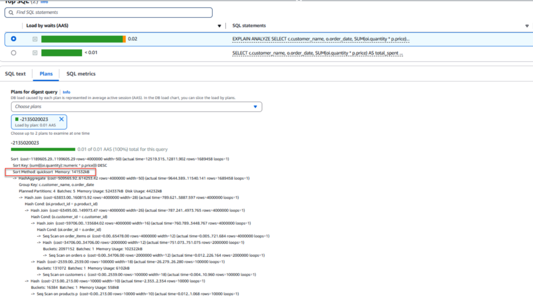
Here is the detail of execution plan as seen in above screenshot.

Execution plan -2135020023

Sort (cost=1189605.29..1199605.29 rows=4000000 width=50) (actual time=12519.315..12811.902 rows=1689458 loops=1)
Sort Key: (sum((oi.quantity)::numeric * p.price))) DESC
Sort Method: quicksort Memory: 141532kB
-> HashAggregate (cost=509565.92..614253.42 rows=4000000 width=50) (actual time=9644.389..11540.141 rows=1689458 loops=1)
Group Key: c.customer_name, o.order_date
Planned Partitions: 4 Batches: 5 Memory Usage: 524288kB Disk Usage: 442432kB
-> Hash Join (cost=63853.00..160815.92 rows=4000000 width=28) (actual time=789.621..5887.597 rows=4000000 loops=1)
Hash Cond: (oi.product_id = p.product_id)
-> Hash Join (cost=63495.00..149973.47 rows=4000000 width=26) (actual time=787.241..4973.765 rows=4000000 loops=1)
Hash Cond: (o.customer_id = c.customer_id)
-> Hash Join (cost=59706.00..135884.02 rows=4000000 width=16) (actual time=760.789..3448.767 rows=4000000 loops=1)
Hash Cond: (order_id = order_id)
-> Seq Scan on order_items oi (cost=0.00..65478.00 rows=4000000 width=12) (actual time=0.005..721.684 rows=4000000 loops=1)
-> Hash (cost=34706.00..34706.00 rows=2000000 width=12) (actual time=751.073..751.075 rows=2000000 loops=1)
Buckets: 2097152 Batches: 1 Memory Usage: 102522kB
-> Seq Scan on orders o (cost=0.00..34706.00 rows=2000000 width=12) (actual time=0.012..226.164 rows=2000000 loops=1)
-> Hash (cost=2539.00..2539.00 rows=100000 width=18) (actual time=26.279..26.280 rows=100000 loops=1)
Buckets: 131072 Batches: 1 Memory Usage: 6102kB
-> Seq Scan on customers c (cost=0.00..2539.00 rows=100000 width=18) (actual time=0.004..10.960 rows=100000 loops=1)
-> Hash (cost=213.00..213.00 rows=10000 width=10) (actual time=2.355..2.354 rows=10000 loops=1)
Buckets: 16384 Batches: 1 Memory Usage: 558kB
-> Seq Scan on products p (cost=0.00..213.00 rows=10000 width=10) (actual time=0.012..1.068 rows=10000 loops=1)

Using CloudWatch Database Insights simplified the optimization process by providing clear visualization of query execution patterns, which helped us identify the work_mem parameter as the root cause.

Conclusion

In this post, we showed how to use CloudWatch Database Insights for Aurora PostgreSQL to analyze execution plan changes and resource constraints that impact database performance, without extensive manual investigation. In our example scenarios, we identified a sudden spike in query latency caused by a dropped index that changed the query’s access path, and diagnosed a performance bottleneck from disk-based sorting operations and resolved it by increasing the work_mem parameter.

Get started with CloudWatch Database Insights.

About the authors