AWS Database Blog
Implement fast, space-efficient lookups using Bloom filters in Amazon ElastiCache
Amazon ElastiCache now supports Bloom filters: a fast, memory-efficient, probabilistic data structure that lets you quickly insert items and check whether items exist. Bloom filters are a powerful tool for many different use cases, such as advertisement and promotional campaign deduplication, fraud detection, filtering harmful content, detecting malicious URLs, checking if usernames are taken, and generally avoiding expensive disk lookups. In this post, we discuss two real-world use cases demonstrating how Bloom filters work in ElastiCache, the best-practices to implement, and how you can save at least 90% in memory and cost compared to alternative implementations. Bloom filters are available in ElastiCache version 8.1 for Valkey in all AWS Regions and at no additional cost.
Introduction to Bloom filters
Bloom filters are a space-efficient probabilistic data structure that supports adding elements and checking whether specific elements were previously added. False positives are possible, where a filter indicates that an element exists even though it wasn’t added. However, Bloom filters prevent false negatives, meaning that an element that was added successfully will not be reported as not existing.
To illustrate the mechanics of Bloom filters, see the following figure (source).

Here, we use K different hash functions that compute K corresponding bits from a bit vector. When adding an item, these bits are set to 1. During existence checking, if a bit is 0, the item is definitively absent. However, if all bits are 1, the item likely exists, with a defined false positive probability. For example, items x, y, and z would show all bits as 1, indicating their likely existence, whereas an item like w would show one bit as 0, definitively proving its absence. This bit-based approach, rather than full item allocation, is what makes Bloom filters highly space-efficient.
The following diagram depicts how Bloom filters are implemented in Valkey as well as key concepts for understanding how Bloom filters are implemented and how to use them.
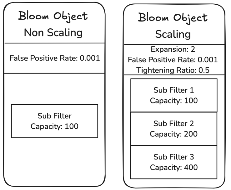
The Bloom object is the primary data structure created with a Bloom filter creation command. It offers two operational modes: non-scaling, which enforces a fixed capacity and returns an error when it’s full, and scaling, which automatically grows by adding new sub-filters when capacity is exceeded. Sub-filters are an inner structure within the Bloom object that have a certain capacity, or number of items it can hold. You can set the capacity for the first sub-filter and then in scaling mode, the expansion rate determines how the capacity of newly created sub-filters grows. You can also configure what false positive rate is acceptable for your workload, which determines how often such false positives occur. Making your Bloom filter more accurate with fewer false positives requires more memory usage, though only marginally, which we demonstrate later in this post.
The Bloom filter solution in ElastiCache uses the valkey-bloom module from the Valkey open-source project and therefore is fully compatible with the open-source module, and it’s API-compatible with the Bloom filter command syntax of the Valkey client libraries, including valkey-py, valkey-java, and valkey-go (as well as the equivalent Redis libraries).
Now that we understand the key concepts of Bloom filters, let’s explore some real-world examples to see how you can use and configure Bloom filters and the value they provide.
Use case #1: Advertisement deduplication
In this example, we look at a common use case of Bloom filters: advertisement deduplication. Applications can use Bloom filters to track whether an advertisement or promotion has already been shown to a customer in order to prevent showing it again to the same customer.
Let’s assume we have 500 unique advertisements that need to be shown. Both advertisements and customers are identified by a UUID (36 characters). For this, we create 500 Bloom filter objects, one representing each advertisement, using the BF.RESERVE or BF.INSERT command. When creating a Bloom filter, we specify the false positive rate, the scaling or non-scaling property, and the capacity. Because we want to maximize customer conversation rates, we must make sure advertisements are being shown to the majority of the customers. Therefore, we set the false positive rate to be low, for example 0.000001, so that no more than 1 in 1 million customers may miss seeing an advertisement that they should be shown. Because Bloom filters make sure false negatives don’t occur, the customer isn’t shown an ad more than one time.
Next, let’s specify the capacity and the scaling property. For this, we need to think about how many items will be inserted into the Bloom filter over time. In this example, let’s say we’re unsure the total number of visits a given advertisement or promotion will get, but we know that it will be at least 10,000. Because we’re unsure about our capacity needs, but we know that it will grow, we should use a scaling Bloom filter. We can set the initial capacity to be 10,000 with an expansion rate of 2. This means that after the Bloom filter’s first sub-filter reaches its capacity, upon a new insertion (when customer 10,001 sees the advertisement), during scale-out, a new sub-filter is added with a capacity that is two times the capacity of the first sub-filter, or 20,000. The Bloom filter then has a total capacity of 30,000. The next sub-filter would have a capacity of 40,000, bringing the total capacity to 70,000, and so forth.
We can create a Bloom filter for our first advertisement with the preceding configuration as follows:
When a customer is shown an advertisement, we can add their customer ID to the corresponding Bloom filter with BF.ADD, or BF.MADD to add more than one customer IDs. To check if they have already seen the advertisement, we use the BF.EXISTS or BF.MEXISTS command.
The following table shows how the capacity grows according to the expansion rate and the corresponding memory used for that capacity.
| Number of Bloom Filters | Capacity per Scaling Bloom Filter (Summed Across Sub-Filters) | Number of Scale-Outs | False Positive Rate | Memory Usage (MB) per Bloom Filter | Total Used Memory (GB) Across 500 Bloom Filters | Cost for Data Stored per Month |
| 500 | 10,000 | 0 | 0.000001 | 0.03 | 0.06 | $3.84 |
| 500 | 30,000 | 1 | 0.000001 | 0.11 | 0.10 | $6.23 |
| 500 | 70,000 | 2 | 0.000001 | 0.26 | 0.18 | $11.01 |
| 500 | 150,000 | 3 | 0.000001 | 0.57 | 0.36 | $22.46 |
| 500 | 310,000 | 4 | 0.000001 | 1.23 | 0.73 | $45.35 |
| 500 | 630,000 | 5 | 0.000001 | 2.60 | 1.46 | $91.24 |
| 500 | 1,270,000 | 6 | 0.000001 | 5.46 | 2.92 | $182.49 |
| 500 | 2,550,000 | 7 | 0.000001 | 11.39 | 5.85 | $365.60 |
| 500 | 5,110,000 | 8 | 0.000001 | 23.69 | 12.96 | $809.95 |
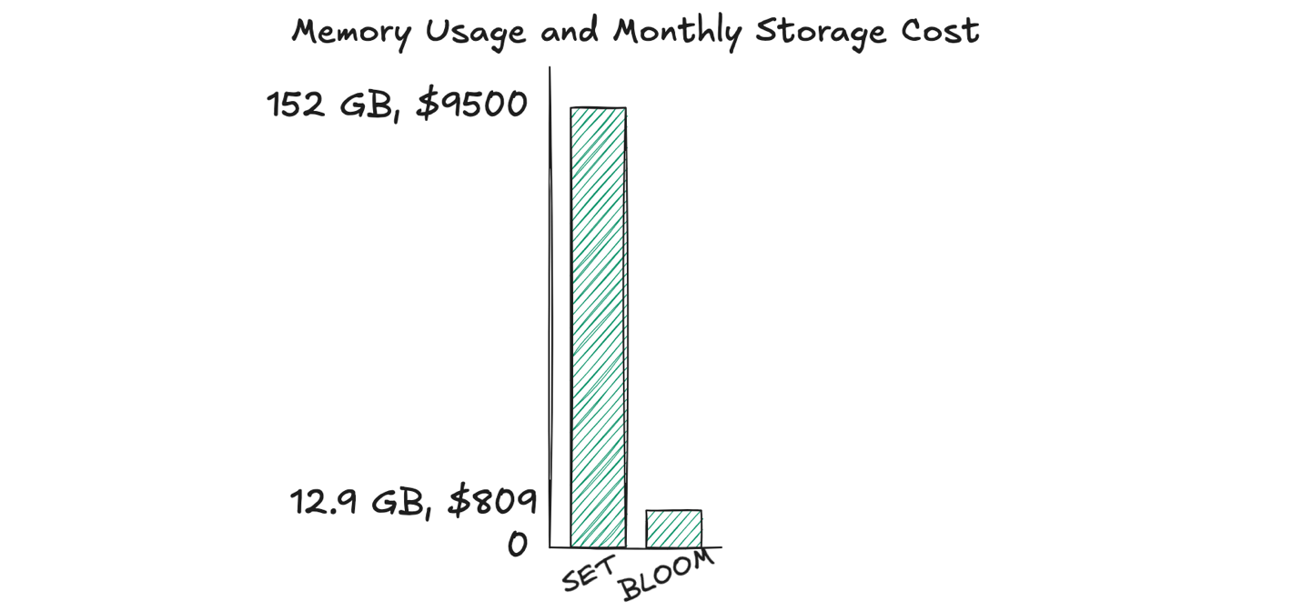
With an expansion rate of 2, by the eighth scale-out, the Bloom filter’s total capacity becomes just over 5 million. To track 5 million customers for each of the 500 advertisements, using the Bloom filter data type, you would need over 12.9 GB of memory on an ElastiCache Valkey 8.0 node for the given false positive rate.
To demonstrate the memory efficiency of Bloom filters and the cost savings that this translates to, let’s compare the same setup using the Set data type. With sets, we create a specific set object for every advertisement and use the SADD command to track every customer who has already seen this particular advertisement by adding them to the set. To check if a customer has seen the ad, we can use the SISMEMBER or SMISMEMBER commands.
To track 5 million customers for each of the 500 advertisements, using the Set data type, you would need over 152 GB of memory on an ElastiCache Valkey 8.0 node. At the time of publishing this blog, based on ElastiCache pricing, using an ElastiCache Serverless Valkey cluster in the us-east-1 Region with data storage of 152 GB costs approximately $9,500 per month. Using scaling Bloom filters for the same workload and scenario costs $809 because it only uses 12.9 GB. In this scenario, using Bloom filters translates to nearly 92% cost savings. With Bloom filters, you can achieve significant memory savings at the cost of potential false positives (which are configurable). This is a great trade-off for some membership testing use cases.
Use case #2: Financial fraud detection
Let’s look at another common use case of Bloom filters: financial fraud detection. Financial institutions can use Bloom filters to track whether a credit card has previously transacted with a specific merchant. In this example, let’s assume we’re a financial institution operating with 100 million credit cards, where each card performs transactions with 10 different merchants. Credit cards are identified by a 16-character unique sequence, and merchants are identified by a 15-character merchant ID.
Similar to the previous example, let’s compare Bloom filters with using the Set data type. With sets, we first hash the cards into 200 buckets to manage the scale by distributing the cards into multiple objects. Each bucket has its own set, and the SADD command is used to track each card-merchant combination by storing a concatenated string of the card number, a colon, and the merchant ID. This is 32 characters total. To check if a card has transacted with a merchant before, we can use the SISMEMBER or SMISMEMBER commands. This means we have 200 sets, each with approximately 5 million members (100 million cards with 10 merchants distributed across 200 buckets/sets). This will require 61 GB of memory.
With Bloom filters, applications can still hash the cards into 200 buckets, and create a unique Bloom filter for each bucket using the BF.RESERVE or BF.INSERT command. In this case, because the number of credit cards is fixed, we can use non-scaling Bloom filters where the capacity for each filter is set to 5 million to accommodate the 10 merchants each card buys from. For each transaction, the application adds the concatenated card ID and merchant ID separated by a colon as an item to the corresponding Bloom filter. To check if a card has purchased from a merchant previously, we can use the BF.EXISTS or BF.MEXISTS commands on the appropriate filter (determined by the card’s hash).
Now let’s consider the false positive rate. When choosing the false positive rate, you must balance the cost or impact to your use case of false positives with the difference in memory savings you will achieve. Let’s use this example to explore how different false positive rates translate to different memory requirements and therefore different cost savings compared to using sets.
We can create a Bloom filter representing the first credit card bucket with the preceding configurations as follows:
With the same cost calculation assumptions as use case 1, for the preceding workload, the 61 GB data storage utilized by the Set data type costs $3,818 for one month. In contrast, using non-scaling Bloom filters for the same workload, the following table shows that accepting a false positive rate of 1%, you can achieve as much as 98% cost savings compared to sets. If you wanted to minimize false positives to 1 in every 5 million, you still get 93% cost savings compared to using sets. Bloom filters are highly efficient even if you are sensitive to false positives.
| Number of Bloom Filters | Capacity per Bloom Filter | False Positive Rate | False Positive Rate Description | Memory Usage (MB) per Bloom Filter | Total Used Memory (GB) Across 200 Bloom Filters | Cost for Data Stored per Month | Cost Saved per Month Compared to sets |
| 200 | 5,000,000 | 0.01 | One in every 100 | 5.71 | 1.21 | $75.62 | $3,742.89 |
| 200 | 5,000,000 | 0.001 | One in every 1,000 | 8.57 | 2.00 | $124.99 | $3,693.51 |
| 200 | 5,000,000 | 0.00001 | One in every 100,000 | 14.28 | 3.17 | $198.11 | $3,620.39 |
| 200 | 5,000,000 | 0.0000002 | One in every 5 million | 19.14 | 3.95 | $246.86 | $3,571.65 |
Best practices
Let’s discuss best practices for Bloom filters on ElastiCache for Valkey.
Large Bloom filters
ElastiCache enforces a 128 MB memory usage limit per Bloom object to improve server performance during serialization and deserialization of Bloom filters. Because scalable Bloom filters can grow and expand over time as items are populated, individual Bloom objects are susceptible to experiencing memory usage errors when attempting to scale out. For example:
You can address this in two ways. First, before implementation, check your capacity requirements and use the BF.INSERT command with the VALIDATESCALETO option to make sure your planned filter capacity, along with other configured properties, fits within the 128 MB memory limit per object. This helps prevent insertion errors later due to memory constraints while maintaining your desired accuracy. In the following example, we see that filter1 can’t scale out and reach the capacity of 26,214,301 due to the memory limit. However, it can scale out and reach a capacity of 26,214,300.
Second, for existing filters, use the BF.INFO command to find out the maximum capacity that your scalable Bloom filter can expand to hold. This helps plan for your application requirements before hitting memory limits. In this case, the filter can hold 26,214,300 items (after scaling out until the memory limit):
The BF.INFO command can also be used on both scalable and non-scaling Bloom filters to check its current usage in terms of number of items inserted, memory usage, and more.
The following table summarizes the maximum capacity of an individual non-scaling filter given the memory limit per object. With a 128 MB limit and default false positive rate, we can create a Bloom filter with 112 million as the capacity.
| Capacity (Non-Scaling Filter) | False Positive Rate |
| 112 million | 0.01 |
| 74.6 million | 0.001 |
| 56 million | 0.0001 |
| 44.8 million | 0.00001 |
| 37.3 million | 0.000001 |
Performance
Understanding Bloom filter performance characteristics helps choose optimal properties during filter creation. The Bloom commands BF.ADD and BF.EXISTS have a time complexity of O(K), where K is the number of hash functions, because they operate on a single item. For Bloom commands operating on N items, such as BF.INSERT, BF.MADD, and BF.MEXISTS, the complexity becomes O(N × K). Commands like BF.CARD, BF.INFO, BF.RESERVE, and BF.INSERT (without items) operate in constant time.
In scalable Bloom filters, each scale-out introduces a new sub-filter, each requiring additional hash function checks for the commands operating on it with items. As the filter scales, the false positive rate of the new sub-filter becomes stricter by default (see tightening ratio), which can increase the number of hash functions. Therefore, when a Bloom object scales out several times (such as more than 100 times), the performance can begin to degrade.
To avoid excessive scale-outs and their performance cost, it’s recommended to choose a suitable starting capacity and expansion rate based on expected workload. For example, to store 10 million items, we can use a starting capacity of 100,000 with expansion rate 1, resulting in 100 sub-filters (after 99 scale-outs). However, we can avoid excessive scale-outs with two approaches:
- Use a higher expansion rate of 2 to achieve 12.7 million items with only 7 sub-filters
- Use a higher starting capacity of 1 million to achieve 10 million items with just 10 sub-filters
Choosing larger initial capacities and higher expansion rates optimizes performance by reducing the sub-filters and hash checks. However, be mindful that overly large starting capacities or high expansion rates might lead to over-provisioned filters, resulting in higher memory usage than necessary if actual data volume falls short.
Conclusion
Bloom filters are a powerful addition to the ElastiCache toolkit, enabling fast, scalable, and space-efficient membership testing across a wide range of applications. As shown in the real-world examples of ad deduplication and fraud detection, Bloom filters deliver dramatic memory savings—often over 90%—by trading off a small, configurable rate of false positives, all without compromising performance. With native support in ElastiCache version 8.1 for Valkey and full compatibility with open source Valkey clients, adopting Bloom filters requires minimal effort and offers immediate value.
Bloom filters are available today in ElastiCache version 8.1 for Valkey in all Regions and for both node-based and serverless offerings. To learn more about Bloom filters on ElastiCache for Valkey, refer to ElastiCache documentation. For the full documentation and list of supported commands, see the Bloom filter documentation on valkey.io.